
Blogg
The Hyperspace theory whith Quantum Field theory
02.05.2014 21:04
The Hyperspace theory whith
Quantum Field theory
In this reworked and extended version of the Hyper space theory I will introduce my 4dimensional quantum field theory that apply in our 4space and in the parallel 4spaces , this theory says that everything is light in 4dimensions because that the formula for the energy of a particle Wp=hf4 is true for every particle in our 4space and not only for photons (corresponding relationship is the case in the parallel 4spaces) massive particles are propably closed waves in 3dimensions (but open waves in the 4:th dimension) that looks like some kind of twistorfield (see the picture ”twistorfield”) and only exists in some quantized frequencies (energies) while light and electrogravitationparticles (photons and gravitophotons) are open waves that can have any frequency.
Constants: Lightspeed in vacuum: c=2,99792458¤108[m/s] ,
Magnetical constant: µ0=4π¤10-7[Vs/Am] ,
Electrical constant ϵ0=8,85418782¤10-12[As/Vm] ,
Planck’s constant: h=6,626076¤10-34[Js].
It exists parallel universes(4spaces) whit higher lightspeed than our own universe , in these universes the standard lightspeed and 4velocity is c’= Nc where c is the standard lightspeed and N is an integer number (whole number) that is called the hyper factor (that is 1 in our universe).
The 4velocity in our universe(4space) in our 4space the following is true:
v2+vct2=vx2+vy2+vz2+vt2=c2 c=(vx;vy;vz;vt)
v2=vx2+vy2+vz2 v=(vx;vy;vz)
in corresponding way the following must be true for the parallel universes:
v’2+v’ct2=v’x2+v’y2+v’z2+v’t2=c’2=N2c2 c’=Nc=(v’x;v’y;v’z;v’t)
v’2=v’x2+v’y2+v’z2=N2v2 v’=(v’x;v’y;v’z)
hence it follows that if the 4velocity has the same direction in our universe as in the parallel universe (which it becomes for an object that is transferred to hyperspace) hence the following is true:
v’/v=v’x/vx=v’y/vy=v’z/vz=v’t/vt=c’/c=N
Hence it follows that v’x=Nvx v’y=Nvy v’z=Nvz v’t=Nvt Where v’ is the space velocity in the parallel universe , v’x is the x-component of the 4velocity in the parallel universe , v’y is the y-component of the 4velocity in the parallel universe , v’z is the z-component of the 4velocity in the parralel universe and v’t is the component of the 4velocity in the time dimension of the parallel universe.
v is the space velocity in our universe , vx is the x-component of the 4velocity in our universe , vy is the y-component of the 4velocity in our universe , vz is the z-component of the 4velocity in our universe and vt is the component of the 4velocity in the time dimension of our universe.
dx’=dx dy’=dy dz’=dz dT’=dT/N dt’=dt/N
Where dx’=dx is the smallest possible length in x-direction in both our universe and in the parrallel universes , where dy’=dy is the smallest possible length in y-direction in both our universe and in the parrallel universes , where dz’=dz is the smallest possible length in z-direction in both our universe and in the parrallel universes , dT’ is the smallest possible own time interval in the parallel universe , dT is the smallest possible own time interval in our universe , dt’ is the smallest possible coordinate time interval in the parallel universe and dt is the smallest possible coordinate time interval in our universe.
mp=qpU/c2=Wp/c2=hf4p/c2=h/(λ4pc)=p4p/c qp=hf4p/U Where mp is the mass of the particle , qp is the charge of the particle, Wp is the energy of the particle, h is planck’s constant , f4p is the 4quantum wave frequency of the particle , λ4p is the 4quantum wavelength of the particle and p4p is the 4momentum of the particle (in standard space).
p3p=mpv=Wpv/c2=qpUv/c2=p4pv/c=hf4pv/c2=(hv)/(λ4pc)=h/λ3p
p4p=mpc=Wp/c=qpU/c=hf4p/c=h/λ4p
pxp=mpvx=Wpvx/c2=qpUvx/c2=p4pvx/c=hf4pvx/c2=(hvx)/(λ4pc)=h/λxp
pyp=mpvy=Wpvy/c2=qpUvy/c2=p4pvy/c=hf4pvy/c2=(hvy)/(λ4pc)=h/λyp
pzp=mpvz=Wpvz/c2=qpUvz/c2=p4pvz/c=hf4pvz/c2=(hvz)/(λ4pc)=h/λzp
pctp=mpvt=Wpvt/c2=qpUvt/c2=p4pvt/c=hf4pvt/c2=(hvt)/(λ4pc)=h/λctp
p3p2=pxp2+pyp2+pzp2 p4p2=p3p2+pctp2=pxp2+pyp2+pzp2+pctp2 p3p=(pxp;pyp;pzp) p4p=(pxp;pyp;pzp;pctp)
Where p3p is the particles momentum in space , pxp is the x-component of the particles momentum , pyp is the y-component of the particles momentum , pzp is the z-component of the particles momentum and pctp is the particles momentum component in the time dimension (in our universe).
λ4p=h/p4p=h/(mpc)=hc/(qpU)=hc/Wp
λ3p=h/p3p=hc/(p4pv)=λ4pc/v
λxp=h/pxp=hc/(p4pvx)=λ4pc/vx
λyp=h/pyp=hc/(p4pvy)=λ4pc/vy
λzp=h/pzp=hc/(p4pvz)=λ4pc/vz
λctp=h/pctp=hc/(p4pvt)=λ4pc/vt
λ3p-2=λxp-2+λyp-2+λzp-2 λ4p-2=λ3p-2+λctp-2=λxp-2+λyp-2+λzp-2+λctp-2
λ3p-1=(λxp-1;λyp-1;λzp-1) λ4p-1=(λxp-1;λyp-1;λzp-1+λctp-1)
Where λ3p is the quantum wavelength of the particle in space , λxp is the quantum wavelength of the particle in x-direction , λyp is the quantum wavelength of the particle in y-direction , λzp is the quantum wavelength of the particle in z-direction and λctp is the quantum wavelength of the particle in the time dimension. As you can see from the equations above the quantum wavelengths inverses are vectors , this also means that for a particle that stands still in space the space wavelength becomes infinite and for a particle that stands still in one dimension the wavelength in this dimension becomes infinite it is in all places in this dimension at once. A possible way to ascend could be that make every particle that is part of you completelly stop moving in space then the particles and youself would get an infinite space wavelength and you would be in all places in this universe simultaneously , if you also would let some particles that is part of you travel with lightspeed in a space dimension these particles would get infinite wavelength in time and in the two space dimensions perpendicular to the direction of travel , if ones consciousness was spread on these particles and totally stillstanding particles whit infinite space wavelengths you would be one whit our 4space that is our universe and be on all places and times simultaneously then you have ascended one level higher.
c=f4pλ4p f4p=c/λ4p=cp4p/h=mpc2/h=qpU/h=Wp/h
v=f3pλ3p f3p=v/λ3p=v2/(λ4pc)=(v2/c2)f4p
vx=fxpλxp fxp=vx/λxp=vx2/(λ4pc)=(vx2/c2)f4p
vy=fypλyp fyp=vy/λyp=vy2/(λ4pc)=(vy2/c2)f4p
vz=fzpλzp fzp=vz/λzp=vz2/(λ4pc)=(vz2/c2)f4p
vt=fctpλctp fctp=vt/λctp=vt2/(λ4pc)=(vt2/c2)f4p
f3p=fxp+fyp+fzp f4p=f3p+fctp=fxp+fyp+fzp+fctp
Where f3p is the quantum wave frequency of the particle in space , fxp is the quantum wave frequency of the particle in x-direction , fyp is the quantum wave frequency of the particle in y-direction , fzp is the quantum wave frequency of the particle in z-direction and fctp is the quantum wave frequency of the particle in the time dimension. ( in our universe) as you see the 4quantum wave frequency is the (scalar) sum of the quantum wave frequensies in the 4dimensions.
Wp=hf4p=qpU=mpc2=p4pc Wp=ctWp+SWp=ctWp+xWp+yWp+zWp
SWp=xWp+yWp+zWp
SWp=Wpv2/c2=mpv2=p3pv=hf3p
xWp=Wpvx2/c2=mpvx2=pxpvx=hfxp
yWp=Wpvy2/c2=mpvy2=pypvy=hfyp
zWp=Wpvz2/c2=mpvz2=pzpvz=hfzp
ctWp=Wpvt2/c2=mpvt2=pctpvt=hfctp
Where SWp is the space motion energy of the particle , xWp is the particles motion energy in x-direction , yWp is the particles motion energy in y-direction , zWp is the particles motion energy in z-direction and ctWp is the time (zero point) energy of the particle (in our universe).
p4=∑p4p=∑(h/λ4p)=∭(ρ0U/c)dxdydz=∭(¤c)dxdydz=W/c
p3=∑p3p=∑(h/λ3p)=∭(ρ0Uv/c2)dxdydz=∭(¤v)dxdydz=∭(Pv/c2)dxdydz
px=∑pxp=∑(h/λxp)=∭(ρ0Uvx/c2)dxdydz=∭(¤vx)dxdydz=∭(Pvx/c2)dxdydz
py=∑pyp=∑(h/λyp)=∭(ρ0Uvy/c2)dxdydz=∭(¤vy)dxdydz=∭(Pvy/c2)dxdydz
pz=∑pzp=∑(h/λzp)=∭(ρ0Uvz/c2)dxdydz=∭(¤vz)dxdydz=∭(Pvz/c2)dxdydz
pct=∑pctp=∑(h/λctp)=∭(ρ0Uvt/c2)dxdydz=∭(¤vt)dxdydz=∭(Pvt/c2)dxdydz
p32=px2+py2+pz2 p42=p32+pct2=px2+py2+pz2+pct2
p3=(px;py;pz) p4=(px;py;pz;pct) P=d3W/(dxdydz)
Where p4 is the 4momentum of an object in standard space , p3 is the momentum of an object in standard space , px is the x-component of the momentum , py is the y-component of the momentum , pz is the z-component of the momentum and pct is the time momentum of an object in standard space and P is the pressure (spacetime energy/volume).
W=∑Wp=∑(hf4p)=∭(ρ0U)dxdydz=∭(¤c2)dxdydz=∫Fxdx+∫Fydy+∫Fzdz+∫Fctcdt
SW=∑SWp=∑hf3p
xW=∑xWp=∑hfxp=∫xFydy+∫xFzdz+∫xFctcdt
yW=∑yWp=∑hfyp=∫yFxdx+∫yFzdz+∫yFctcdt
zW=∑zWp=∑hfzp=∫zFxdx+∫zFydy+∫zFctcdt
ctW=∑ctWp=∑hfctp=∫ctFxdx+∫ctFydy+∫ctFzdz
SW=xW+yW+zW W=SW+ctW=xW+yW+zW+ctW
Where W is the energy of an object , SW is the space motion energy of an object , xW is the motion energy of an object in x-direction , yW is the motion energy of an object in y-direction , zW is the motion energy of an object in z-direction and ctW is the time (zero point) energy of an object (in our universe).
F4p=dp4p/dT=d(mpc)/dT=mp(dc/dT)+c(dmp/dT) F4p=qpE4
F3p=dp3p/dT=d(mpv)/dT=mp(dv/dT)+v(dmp/dT) F3p=qpE3
Fxp=dpxp/dT=d(mpvx)/dT=mp(dvx/dT)+vx(dmp/dT) Fxp=qpEx=qp(∫(d(Esxcdt)/cdT)-∫(d(Byxdy)/dT-∫(d(Bzxdz)/dT=qp(vtEsx/c+∫(dEsx/(cdT))cdt-vyByx-∫(dByx/dT)dy-vzBzx-∫(dBzx/dT)dz)
Fyp=dpyp/dT=d(mpvy)/dT=mp(dvy/dT)+vy(dmp/dT) Fyp=qpEy=qp(∫(d(Esycdt)/cdT)-∫(d(Bxydx)/dT-∫(d(Bzydz)/dT=qp(vtEsy/c+∫(dEsy/(cdT))cdt-vxBxy-∫(dBxy/dT)dx-vzBzy-∫(dBzy/dT)dz)
Fzp=dpzp/dT=d(mpvz)/dT=mp(dvz/dT)+vz(dmp/dT) Fzp=qpEz=qp(∫(d(Eszcdt)/cdT)-∫(d(Bxzdx)/dT-∫(d(Byzdy)/dT=qp(vtEsz/c+∫(dEsz/(cdT))cdt-vxBxz-∫(dBxz/dT)dx-vyByz-∫(dByz/dT)dy)
Fctp=dpctp/dT=d(mpvt)/dT=mp(dvt/dT)+vt(dmp/dT) Fctp=qpEct=qp(∫(d(Bxctdx)/dT)+∫(d(Byctdy)/dT+∫(d(Bzctdz)/dT=qp(vxBxct+∫(dBxct/dT)dx+vyByct+∫(dByct/dT)dy+vzBzct+∫(dBzct/dT)dz)
F3p2=Fxp2+Fyp2+Fzp2 F4p2=F3p2+Fctp2=Fxp2+Fyp2+Fzp2+Fctp2
F3p=(Fxp;Fyp;Fzp) F4p=(Fxp;Fyp;Fzp;Fctp)
Where F4p is the force on the particle and F3p is the force on the particle in the space dimensions , Fxp is the x-component of the force on the particle , Fyp is the y-component of the force on the particle , Fzp is the z-component of the force on the particle and Fctp is the time component of the force on the particle (in our universe).
F4=∑F4p=dp4/dT=∭(d(¤c)/dT)dxdydz=∭(¤(dc/dT))dxdydz+∭(c(d¤/dT))dxdydz F4=∭(ρ0E4)dxdydz
F3=∑F3p=dp3/dT=∭(d(¤v)/dT)dxdydz=∭(¤(dv/dT))dxdydz+∭(v(d¤/dT))dxdydz F3=∭(ρ0E3)dxdydz
Fx=∑Fxp=dpx/dT=∭(d(¤vx)/dT)dxdydz=∭(¤(dvx/dT))dxdydz+∭(vx(d¤/dT))dxdydz Fx=ctFx+yFx+zFx=∭(ρ0Ex)dxdydz=∭(ρ0(vtEsx/c+∫(dEsx/(cdT))cdt-∫(dByx/dT)dy-∫(dBzx/dT)dz)dxdydz-∭(jyByx)dxdydz-∭(jzBzx)dxdydz
Fy=∑Fyp=dpy/dT=∭(d(¤vy)/dT)dxdydz=∭(¤(dvy/dT))dxdydz+∭(vy(d¤/dT))dxdydz Fy=ctFy+xFy+zFy=∭(ρ0Ey)dxdydz=∭(ρ0(vtEsy/c+∫(dEsy/(cdT))cdt-∫(dBxy/dT)dx-∫(dBzy/dT)dz)dxdydz-∭(jxBxy)dxdydz-∭(jzBzy)dxdydz
Fz=∑Fzp=dpz/dT=∭(d(¤vz)/dT)dxdydz=∭(¤(dvz/dT))dxdydz+∭(vz(d¤/dT))dxdydz Fz=ctFz+xFz+yFz=∭(ρ0Ez)dxdydz=∭(ρ0(vtEsz/c+∫(dEsz/(cdT))cdt-∫(dBxz/dT)dx-∫(dByz/dT)dy)dxdydz-∭(jxBxz)dxdydz-∭(jyByz)dxdydz
Fct=∑Fctp=dpct/dT=∭(d(¤vt)/dT)dxdydz=∭(¤(dvt/dT))dxdydz+∭(vt(d¤/dT))dxdydz Fct=xFct+yFct+zFct=∭(ρ0Ect)dxdydz=∭(ρ0(∫(dBxct/dT)dx +∫(dByct/dT)dy+∫(dBzct/dT)dz)dxdydz+∭(jxBxct)dxdydz+∭(jyByct)dxdydz+∭(jzBzct)dxdydz
F32=Fx2+Fy2+Fz2 F42=F32+Fct2=Fx2+Fy2+Fz2+Fct2
F3=(Fx;Fy;Fz) F4=(Fx;Fy;Fz;Fct)
Where F4 is the force and F3 is the force in the space dimensions , Fx is the x-component of the force , Fy is the y-component of the force , Fz is the z-component of the force and Fct is the force component in the time dimension (in our universe) E4 is the 4dimensional electrical field , E3 is the electrical field in the space dimensions , Ex is the x-component of the electric field , Ey is the y-component of the electric field , Ez is the z-component of the electric field , Ect is the electrical field in the time dimension , jx is the x-component of the current density , jy is the y-component of the current density , jz is the z-component of the current density , ¤ is the mass density and ρ0 is the charge density , Esx/c is the electrostatical field/c in x-direction , Esy/c is the electrostatical field/c in y-direction , Esz/c is the electrostatical field/c in z-direction , Bxy is the magnetical field in the y-direction from currents flowing in x-direction , Bxz is the magnetical field in the z-direction from currents flowing in x-direction , Byx is the magnetical field in the x-direction from currents flowing in y-direction , Byz is the magnetical field in the z-direction from currents flowing in y-direction , Bzx is the magnetical field in the x-direction from currents flowing in z-direction , Bzy is the magnetical field in the y-direction from currents flowing in z-direction (all magnetical fields is whit straight field lines , for translation to classical ring-shaped field lines see ”comparison between euclidean 4dimensional electromagnetism and common electromagnetism”) Bxct is the magnetical field in the time dimension from currents flowing in x-direction , Byct is the magnetical field in the time dimension from currents flowing in y-direction and Bzct is the magnetical field in the time dimension from currents flowing in z-direction (in our universe).
Below the corresponding equations for the parallel 4spaces comes , after that I will talk about photon and gravitophoton emission and capture to explain force effect between charges and electrogravitation and transfer to hyperspace.
m’p=q’pU’/c’2=W’p/c’2=h’f*4p/c’2=h’/(λ4pc’)=p’4p/c’ q’p=h’f*4p/U’
Where m’p is the mass of the particle , q’p is the charge of the particle , W’p is the energy of the particle , h’=h/N is the equivalent of planck’s constant in hyperspace , f*4p is the 4quantum wave frequency of the particle , λ4p is the 4quantum wavelength of the particle and p’4p is the 4momentum of the particle (in hyperspace). Derivation of quantities in hyperspace: because c’=Nc and λ’=λ and Wp’=Wp and U’=NU (this is derived later in the article) becomes
c’=f*λ and c=fλ becomes f=c/λ and f*=c’/λ=Nc/λ=Nf f*=Nf Nc=Nfλ
Wp=hf and Wp=h’f* becomes h’=hf/f*=hf/Nf=h/N h’=h/N
Wp=mpc2 and Wp=m’pc’2 becomes m’p=mpc2/c’2=mpc2/(N2c2)=mp/N2 m’p=mp/N2
Wp=qpU and Wp=q’pU’ becomes q’p=qpU/U’=qpU/(NU)=qp/N q’p=qp/N
Where λ=λ’ is the 4quantum wavelength in both our universe and the hyperspace and f is the frequency in our universe and f* is the frequency in the hyperspace (It is because f*=Nf that the hyperspace is called the higher vibrations of reality or the cosmic overtones) U is the electrical potential in our universe and U’ is the electrical potential in the hyperspace.
p’3p=m’pv’=Wpv’/c’2=q’pU’v’/c’2=p’4pv’/c’=h’f*4pv’/c’2=(h’v’)/(λ4pc’)=h’/λ3p=p3p/N p’3p=p3p/N
p’4p=m’pc’=W’p/c’=q’pU’/c’=h’f*4p/c’=h’/λ4p=p4p/N
p’xp=m’pv’x=Wpv’x/c’2=q’pU’v’x/c’2=p’4pv’x/c’=h’f*4pv’x/c’2=(h’v’x)/(λ4pc’)=h’/λxp=pxp/N p’xp=pxp/N
p’yp=m’pv’y=Wpv’y/c’2=q’pU’v’y/c’2=p’4pv’y/c’=h’f*4pv’y/c’2=(h’v’y)/(λ4pc’)=h’/λyp=pyp/N p’yp=pyp/N
p’zp=m’pv’z=Wpv’z/c’2=q’pU’v’z/c’2=p’4pv’z/c’=h’f*4pv’z/c’2=(h’v’z)/(λ4pc’)=h’/λzp=pzp/N p’zp=pzp/N
p’ctp=m’pv’t=W’pv’t/c’2=q’pU’v’t/c’2=p’4pv’t/c’=h’f*4pv’t/c’2=(h’v’t)/(λ4pc’)=h’/λctp=pctp/N p’ctp=pctp/N
p’3p2=p’xp2+p’yp2+p’zp2 p’4p2=p’3p2+p’ctp2=p’xp2+p’yp2+p’zp2+p’ctp2 p’3p=(p’xp;p’yp;p’zp) p’4p=(p’xp;p’yp;p’zp;p’ctp) p’4p=p4p/N
Where p’3p is the momentum of the particle in the space dimensions , p’xp is the x-component of the momentum of the particle , p’yp is the y-component of the momentum of the particle , p’zp is the z-component of the momentum of the particle and p’ctp is the particles momentum component in the time dimension (in hyperspace). You can see from this that the momentum in hyperspace is equivalent to corresponding momentum in standard space/N
λ’4p=h’/p’4p=h’/(m’pc’)=h’c’/(q’pU’)=h’c’/Wp=hN/(Np4p)=h/p4p=λ4p λ’4p=λ4p
λ’3p=h’/p’3p=h’c’/(p’4pv’)=λ4pc’/v’=λ4pNc/(Nv)=λ4pc/v=λ3p λ’3p=λ3p
λ’xp=h’/p’xp=h’c’/(p’4pv’x)=λ4pc’/v’x=λ4pNc/(Nvx)=λ4pc/vx=λxp λ’xp=λxp
λ’yp=h’/p’yp=h’c’/(p’4pv’y)=λ4pc’/v’y=λ4pNc/(Nvy)=λ4pc/vy=λyp λ’yp=λyp
λ’zp=h’/p’zp=h’c’/(p’4pv’z)=λ4pc’/v’z=λ4pNc/(Nvz)=λ4pc/vz=λzp λ’zp=λzp
λ’ctp=h’/p’ctp=h’c’/(p’4pv’t)=λ4pc’/v’t=λ4pNc/(Nvt)=λ4pc/vt=λctp λ’ctp=λctp
λ’3p-2=λ’xp-2+λ’yp-2+λ’zp-2 λ’4p-2=λ’3p-2+λ’ctp-2=λ’xp-2+λ’yp-2+λ’zp-2+λ’ctp-2
λ’3p-1=(λ’xp-1;λ’yp-1;λ’zp-1) λ’4p-1=(λ’xp-1;λ’yp-1;λ’zp-1+λ’ctp-1)
Where λ’3p is the quantum wavelength of the particle in space , λ’xp is the quantum wavelength of the particle in x-direction , λ’yp is the quantum wavelength of the particle in y-direction , λ’zp is the quantum wavelength of the particle in z-direction and λ’ctp is the quantum wavelength of the particle in the time dimension (in hyperspace). As you can see from the equations above the quantum wavelength in hyperspace is the same as corresponding quantum wavelength in standard space. If you transfer particles to all the parallel 4spaces and have left some in our universe and let there be at least two particles in every 4space one completely stillstanding and one that is moving whit the lightspeed of the 4space in one of the space dimensions then you would in every 4space have one particle that has infinite wavelength in space (is on every place at once) and one particle that has infinite wavelength in time dimension and the dimensions perpendicular to the direction of motion (is in every time at once) , If you let one’s consciousness to be spread across all of these particles one will be on all places and times in all 4spaces at once , one has become one whit the cosmos and have ascended to the highest level.
c’=f*4pλ4p f*4p=c’/λ4p=c’p’4p/h’=m’pc’2/h’=q’pU’/h’=W’p/h’=Nc/λ4p=Nf4p f*4p=Nf4p
v’=f*3pλ3p f*3p=v’/λ3p=v’2/(λ4pc’)=(v’2/c’2)f*4p=((Nv)2/(Nc)2)Nf4p=(v2/c2)Nf4p=Nf3p f*3p=Nf3p
v’x=f*xpλxp f*xp=v’x/λxp=v’x2/(λ4pc’)=(v’x2/c’2)f*4p=((Nvx)2/(Nc)2)Nf4p=(vx2/c2)Nf4p=Nfxp f*xp=Nfxp
v’y=f*ypλyp f*yp=v’y/λyp=v’y2/(λ4pc’)=(v’y2/c’2)f*4p=((Nvy)2/(Nc)2)Nf4p=(vy2/c2)Nf4p=Nfyp f*yp=Nfyp
v’z=f*zpλzp f*zp=v’z/λzp=v’z2/(λ4pc’)=(v’z2/c’2)f*4p=((Nvz)2/(Nc)2)Nf4p=(vz2/c2)Nf4p=Nfzp f*zp=Nfzp
v’t=f*ctpλctp f*ctp=v’t/λctp=v’t2/(λ4pc’)=(v’t2/c’2)f*4p=((Nvt)2/(Nc)2)Nf4p=(vt2/c2)Nf4p=Nfctp f*ctp=Nfctp
f*3p=f*xp+f*yp+f*zp f*4p=f*3p+f*ctp=f*xp+f*yp+f*zp+f*ctp
Where f*3p is the quantum wave frequency of the particle in space , f*xp is the quantum wave frequency of the particle in x-direction , f*yp is the quantum wave frequency of the particle in y-direction , f*zp is the quantum wave frequency of the particle in z-direction and f*ctp is the quantum wave frequency of the particle in the time dimension. ( in hyperspace) Even here the 4frequency is the (scalar) sum of the frequencies in the 4 dimensions in the parallel 4space. Of these equations you can see that the frequency in the hyperspace är is the hyper factor times corresponding frequency in our universe and because of that the hyperspace is often called the cosmic overtones or the higher vibrations of reality.
W’p=h’f*4p=q’pU’=m’pc’2=p’4pc’=Wp W’p=Wp W’p=ctW’p+SW’p=ctW’p+xW’p+yW’p+zW’p
SW’p=xW’p+yW’p+zW’p
SW’p=W’pv’2/c’2=m’pv’2=p’3pv’=h’f*3p=SWp SW’p=SWp
xW’p=W’pv’x2/c’2=m’pv’x2=p’xpv’x=h’f*xp=xWp xW’p=xWp
yW’p=W’pv’y2/c’2=mpv’y2=p’ypv’y=h’f*yp=yWp yW’p=yWp
zW’p=W’pv’z2/c’2=m’pv’z2=p’zpv’z=h’f*zp=zWp zW’p=zWp
ctW’p=W’pv’t2/c’2=m’pv’t2=p’ctpv’t=h’f*ctp=ctWp ctW’p=ctWp
Where SW’p is the space motion energy of the particle , xW’p is the particles motion energy in x-direction , yW’p is the particles motion energy in y-direction , zW’p is the particles motion energy in z-direction and ctW’p is the time (zero point) energy of the particle. (in hyperspace) As you can see from the equations the energy of a particle in hyperspace is the same as the energy for an identical particle in standard space.
p’4=∑p’4p=∑(h’/λ4p)=∭(ρ’0U’/c’)dxdydz=∭(¤’c’)dxdydz=W/c’=p4/N p’4=p4/N
p’3=∑p’3p=∑(h’/λ3p)=∭(ρ’0U’v’/c’2)dxdydz=∭(¤’v’)dxdydz=∭(P’v’/c’2)dxdydz=p3/N p’3=p3/N
p’x=∑p’xp=∑(h’/λxp)=∭(ρ’0U’v’x/c’2)dxdydz=∭(¤’v’x)dxdydz=∭(P’v’x/c’2)dxdydz=px/N p’x=px/N
p’y=∑p’yp=∑(h’/λyp)=∭(ρ’0U’v’y/c’2)dxdydz=∭(¤’v’y)dxdydz=∭(P’v’y/c’2)dxdydz=py/N p’y=py/N
p’z=∑p’zp=∑(h’/λzp)=∭(ρ’0U’v’z/c’2)dxdydz=∭(¤’v’z)dxdydz=∭(P’v’z/c’2)dxdydz=pz/N p’z=pz/N
p’ct=∑p’ctp=∑(h’/λctp)=∭(ρ’0U’v’t/c’2)dxdydz=∭(¤’v’t)dxdydz=∭(P’v’t/c’2)dxdydz=pct/N p’ct=pct/N
p’32=p’x2+p’y2+p’z2 p’42=p’32+p’ct2=p’x2+p’y2+p’z2+p’ct2
p’3=(p’x;p’y;p’z) p’4=(p’x;p’y;p’z;p’ct) P’=d3W’/(dxdydz)=P P’=P
Where p’4 is the 4momentum of an object in hyperspace , p’3 is the momentum of an object in hyperspace , p’x is the x-component of the momentum , p’y is the y-component of the momentum , p’z is the z-component of the momentum and p’ct is the time momentum of an object in hyperspace and P’=P is the pressure (spacetime energy/volume) in hyperspace that is the same as in standard space. As you can see the momentum for a system in hyperspace is equivalent whit (the momentum for an identical system in standard space)/N
W’=∑W’p=∑(h’f*4p)=∭(ρ’0U’)dxdydz=∭(¤’c’2)dxdydz=∫F’xdx+∫F’ydy+∫F’zdz+∫F’ctc’dt’=W W’=W
SW’=∑SW’p=∑h’f*3p=SW SW’=SW
xW’=∑xW’p=∑h’f*xp=∫xF’ydy+∫xF’zdz+∫xF’ctc’dt’=xW xW’=xW
yW’=∑yW’p=∑h’f*yp=∫yF’xdx+∫yF’zdz+∫yF’ctc’dt’=yW yW’=yW
zW’=∑zW’p=∑h’f*zp=∫zF’xdx+∫zF’ydy+∫zF’ctc’dt’=zW zW’=zW
ctW’=∑ctW’p=∑h’f*ctp=∫ctF’xdx+∫ctF’ydy+∫ctF’zdz=ctW ctW’=ctW
SW=xW+yW+zW W=SW+ctW=xW+yW+zW+ctW
Where W’ is the energy of an object , SW’ is the space motion energy of an object , xW’ is the motion energy of an object in x-direction , yW’ is the motion energy of an object in y-direction , zW’ is the motion energy of an object in z-direction and ctW’ is the time (zero point) energy of an object (in hyperspace). As you can see from the equations above the energy for a system in hyperspace is equal to the energy for an identical system in standard space.
F’4p=dp’4p/dT’=d(m’pc’)/dT’=m’p(dc’/dT’)+c’(dm’p/dT’)=(dp4p/N)/(dT/N)=dp4p/dT=F4p F’4p=q’pE’4=(qp/N)NE4=qpE4=F4p F’4p=F4p
F’3p=dp’3p/dT’=d(m’pv’)/dT’=m’p(dv’/dT’)+v’(dm’p/dT’)=(dp3p/N)/(dT/N)=dp3p/dT=F3p F’3p=q’pE’3=(qp/N)NE3=qpE3=F3p F’3p=F3p
F’xp=dp’xp/dT’=d(m’pv’x)/dT’=m’p(dv’x/dT’)+v’x(dm’p/dT)=(dpxp/N)/(dT/N)=dpxp/dT=Fxp F’xp=q’pE’x=q’p(∫(d(E’sxc’dt’)/c’dT’)-∫(d(Byxdy)/dT’-∫(d(Bzxdz)/dT’=q’p(v’tE’sx/c’+∫(dE’sx/(c’dT’))c’dt’-v’yByx-∫(dByx/dT’)dy-v’zBzx-∫(dBzx/dT’)dz)=(qp/N)NEx=qpEx=Fxp F’xp=Fxp
F’yp=dp’yp/dT’=d(m’pv’y)/dT’=m’p(dv’y/dT’)+v’y(dm’p/dT’)=(dpyp/N)/(dT/N)=dpyp/dT=Fyp F’yp=q’pE’y=q’p(∫(d(E’syc’dt’)/c’dT’)-∫(d(Bxydx)/dT’-∫(d(Bzydz)/dT’=q’p(v’tE’sy/c’+∫(dE’sy/(c’dT’))c’dt’-v’xBxy-∫(dBxy/dT’)dx-v’zBzy-∫(dBzy/dT’)dz)=(qp/N)NEy=qpEy=Fyp F’yp=Fyp
F’zp=dp’zp/dT’=d(m’pv’z)/dT’=m’p(dv’z/dT’)+v’z(dm’p/dT’)=(dpzp/N)/(dT/N)=dpzp/dT=Fzp F’zp=q’pE’z=q’p(∫(d(E’szc’dt’)/c’dT’)-∫(d(Bxzdx)/dT’-∫(d(Byzdy)/dT’=q’p(v’tE’sz/c’+∫(dE’sz/(c’dT’))c’dt’-v’xBxz-∫(dBxz/dT’)dx-v’yByz-∫(dByz/dT’)dy)=(qp/N)NEz=qpEz=Fzp F’zp=Fzp
F’ctp=dp’ctp/dT’=d(m’pv’t)/dT’=m’p(dv’t/dT’)+v’t(dm’p/dT’)=(dpctp/N)/(dT/N)=dpctp/dT=Fctp F’ctp=q’pE’ct=q’p(∫(d(Bxctdx)/dT’)+∫(d(Byctdy)/dT’+∫(d(Bzctdz)/dT’=q’p(v’xBxct+∫(dBxct/dT’)dx+v’yByct+∫(dByct/dT’)dy+v’zBzct+∫(dBzct/dT’)dz)=(qp/N)NEct=qpEct=Fctp F’ctp=Fctp
F’3p2=F’xp2+F’yp2+F’zp2 F’4p2=F’3p2+F’ctp2=F’xp2+F’yp2+F’zp2+F’ctp2
F’3p=(F’xp;F’yp;F’zp) F’4p=(F’xp;F’yp;F’zp;F’ctp)
Where F’4p is the force on the particle and F’3p is the force on the particle in the space dimensions , F’xp is the x-component of the force on the particle , F’yp is the y-component of the force on the particle , F’zp is the z-component of the force on the particle and F’ctp is the time component of the force on the particle. (in hyperspace) As you can see from the equations the force on a particle in hyperspace is the same as the force on an identical particle in standard space.
F’4=∑F’4p=dp’4/dT’=∭(d(¤’c’)/dT’)dxdydz=∭(¤’(dc’/dT’))dxdydz+∭(c’(d¤’/dT’))dxdydz=(dp4/N)/(dT/N)=dp4/dT=F4 F’4=∭(ρ’0E’4)dxdydz=∭((ρ0/N)NE4)dxdydz=∭(ρ0E4)dxdydz=F4 F’4=F4
F’3=∑F’3p=dp’3/dT’=∭(d(¤’v’)/dT’)dxdydz=∭(¤’(dv’/dT’))dxdydz+∭(v’(d¤’/dT’))dxdydz=(dp3/N)/(dT/N)=dp3/dT=F3 F’3=∭(ρ’0E’3)dxdydz=∭((ρ0/N)NE3)dxdydz=∭(ρ0E3)dxdydz=F3 F’3=F3
F’x=∑F’xp=dp’x/dT’=∭(d(¤’v’x)/dT’)dxdydz=∭(¤’(dv’x/dT’))dxdydz+∭(v’x(d¤’/dT’))dxdydz=(dpx/N)/(dT/N)=dpx/dT=Fx F’x=ctF’x+yF’x+zF’x=∭(ρ’0E’x)dxdydz=∭(ρ’0(v’tE’sx/c’+∫(dE’sx/(’cdT’))c’dt’-∫(dByx/dT’)dy-∫(dBzx/dT’)dz)dxdydz-∭(jyByx)dxdydz-∭(jzBzx)dxdydz=∭((ρ0/N)NEx)dxdydz=∭(ρ0Ex)dxdydz=Fx F’x=Fx
F’y=∑F’yp=dp’y/dT’=∭(d(¤’v’y)/dT’)dxdydz=∭(¤’(dv’y/dT’))dxdydz+∭(v’y(d¤’/dT’))dxdydz=(dpy/N)/(dT/N)=dpy/dT=Fy F’y=ctF’y+xF’y+zF’y=∭(ρ’0E’y)dxdydz=∭(ρ’0(v’tE’sy/c’+∫(dE’sy/(c’dT’))c’dt’-∫(dBxy/dT’)dx-∫(dBzy/dT’)dz)dxdydz-∭(jxBxy)dxdydz-∭(jzBzy)dxdydz=∭((ρ0/N)NEy)dxdydz=∭(ρ0Ey)dxdydz=Fy F’y=Fy
F’z=∑F’zp=dp’z/dT’=∭(d(¤’v’z)/dT’)dxdydz=∭(¤’(dv’z/dT’))dxdydz+∭(v’z(d¤’/dT’))dxdydz=(dpz/N)/(dT/N)=dpz/dT=Fz F’z=ctF’z+xF’z+yF’z=∭(ρ’0E’z)dxdydz=∭(ρ’0(v’tE’sz/c’+∫(dE’sz/(c’dT’))c’dt’-∫(dBxz/dT’)dx-∫(dByz/dT’)dy)dxdydz-∭(jxBxz)dxdydz-∭(jyByz)dxdydz=∭((ρ0/N)NEz)dxdydz=∭(ρ0Ez)dxdydz=Fz F’z=Fz
F’ct=∑F’ctp=dp’ct/dT’=∭(d(¤’v’t)/dT’)dxdydz=∭(¤’(dv’t/dT’))dxdydz+∭(v’t(d¤’/dT’))dxdydz=(dpct/N)/(dT/N)=dpct/dT=Fct F’ct=xF’ct+yF’ct+zF’ct=∭(ρ’0E’ct)dxdydz=∭(ρ’0(∫(dBxct/dT’)dx +∫(dByct/dT’)dy+∫(dBzct/dT’)dz)dxdydz+∭(jxBxct)dxdydz+∭(jyByct)dxdydz+∭(jzBzct)dxdydz=∭((ρ0/N)NEct)dxdydz=∭(ρ0Ect)dxdydz=Fct F’ct=Fct
F’32=F’x2+F’y2+F’z2 F’42=F’32+F’ct2=F’x2+F’y2+F’z2+F’ct2
F’3=(F’x;F’y;F’z) F’4=(F’x;F’y;F’z;F’ct)
Where F’4 is the force and F’3 is the force in the space dimensions , F’x is the x-component of the force , F’y is the y-component of the force , F’z is the z-component of the force and F’ct is the force component in the time dimension (in hyperspace) E’4=NE4 is the 4dimensional electrical field in hyperspace , E’3=NE3 is the electrical field in the space dimensions of the hyperspace , E’x=NEx is the x-component of the electrical field in hyperspace , E’y=NEy is the y-component of the electrical field in hyperspace , E’z=NEz is the z-component of the electrical field in hyperspace , E’ct=NEct is the electrical field in the time dimension of the hyperspace. Of the equations above you can see that the forces on a system in hyperspace becomes the same as for an identical system in standard space.
The energy for an object that is transferred to hyperspace must be the same after the transfer as before (but strangely enough not under the very transfer itself) W’=W where W is the energy of an object
W=∑Wp=∑hf4p=∭(ρ0U)dxdydz=∭(¤c2)dxdydz
W’=∑W’p=∑h’f*4p=∭(ρ’0U’)dxdydz=∭(¤’c’2)dxdydz
Because W’=W so must ¤c2=¤’c’2=¤’N2c2 and ¤’=¤/N2
m’=∭(¤’)dxdydz=∭(¤/N2)dxdydz=m/N2
m=∭(¤)dxdydz
U’=NU
ρ0U=ρ’0U’=ρ’0NU ρ’0=ρ0/N
Q’=∭(ρ’0)dxdydz=∭(ρ0/N)dxdydz=Q/N
Q=∭(ρ0)dxdydz
Where m is the mass of an object in our universe , ¤ is the mass density , Q is the charge of an object and ρ0 is the charge density in our universe and where m’ is the mass of an object in the parallel universe , ¤’ is the mass density , Q’ is the charge of an object and ρ’0 is the charge density in the parallel universe.
E’4=NE4 where E’4 is the electrical field in the parallel 4space and E4 is the electrical field in our 4space
E’32=E’x2+E’y2+E’z2 E’3=(E’x;E’y;E’z) E’3=NE3
E’42=E’32+E’ct2=E’x2+E’y2+E’z2+E’ct2 E’=(E’x;E’y;E’z;E’ct)
U=Ux+Uy+Uz+Uct=∫Exdx+∫Eydy+∫Ezdz+∫Ectcdt=∫(d(Uscdt)/(cdT))-∫(d(Axdx)/dT)-∫(d(Aydy)/dT)-∫(d(Azdz)/dT)=vtUs/c+∫(dUs/(cdT))cdt-vxAx-∫(dAx/dT)dx-vyAy-∫(dAy/dT)dy-vzAz-∫(dAz/dT)dz=vtµ0∬(ρ0vt)((dx)2+(dy)2+(dz)2)+µ0∫(d(∬(ρ0vt)((dx)2+(dy)2+(dz)2))/dT)cdt-vxµ0∬jx((dy)2+(dz)2-(cdt)2-µ0∫(d(∬jx((dy)2+(dz)2-(cdt)2))/dT)dx-vyµ0∬jy((dx)2+(dz)2-(cdt)2-µ0∫(d(∬jy((dx)2+(dz)2-(cdt)2))/dT)dy-vzµ0∬jz((dx)2+(dy)2-(cdt)2-µ0∫(d(∬jz((dx)2+(dy)2-(cdt)2))/dT)dz
U’=U’x+U’y+U’z+U’ct=∫E’xdx+∫E’ydy+∫E’zdz+∫E’ctc’dt’=∫(d(U’sc’dt’)/(c’dT’))-∫(d(Axdx)/dT’)-∫(d(Aydy)/dT’)-∫(d(Azdz)/dT’)=v’tU’s/c’+∫(dU’s/(c’dT’))c’dt’-v’xAx-∫(dAx/dT’)dx-v’yAy-∫(dAy/dT’)dy-v’zAz-∫(dAz/dT’)dz=v’tµ0∬(ρ’0v’t)((dx)2+(dy)2+(dz)2)+µ0∫(d(∬(ρ’0v’t)((dx)2+(dy)2+(dz)2))/dT’)c’dt’-v’xµ0∬jx((dy)2+(dz)2-(c’dt’)2-µ0∫(d(∬jx((dy)2+(dz)2-(c’dt’)2))/dT’)dx-v’yµ0∬jy((dx)2+(dz)2-(c’dt’)2-µ0∫(d(∬jy((dx)2+(dz)2-(c’dt’)2))/dT’)dy-vzµ0∬jz((dx)2+(dy)2-(c’dt’)2-µ0∫(d(∬jz((dx)2+(dy)2-(c’dt’)2))/dT’)dz=NU
U’=NU
Where U is the electrical potential in our 4space and U’ is the electrical potential in the parallel 4space.
µ0=µ’0 the magnetical constant is the same in hyperspace as in our 4space.
c2=1/(ϵ0μ0) c’2=1/(ϵ’0μ0) ϵ0=1/(µ0c2) ϵ’0=1/(µ0c’2)=1/(µ0(Nc)2)=ϵ0/N2 ϵ’0=ϵ0/N2
Where ϵ0 is the electrical constant in our universe and ϵ’0 is the electrical constant in hyperspace.
I is the current in our 4space and I’ is the current in the parallel 4space. (the current in hyperspace is the same as equivalent current in standard space)
I=dQ/dT I’=dQ’/dT’=(dQ/N)/(dT/N)=I I’=I
Below I will derive why magnetic fields , current densities and magnetical vector potential must be the same in hyperspace as in standard space.
jx=ρ0vx jy=ρ0vy jz=ρ0vz j2=jx2+jy2+jz2 j=(jx;jy;jz)
j42=j2+(ρovt)2= jx2+jy2+jz2+(ρ0vt)2 j4=(jx;jy;jz;(ρ0vt))
j’x=ρ’0v’x=(ρ0/N)Nvx=ρ0vx=jx j’x=jx j’y=ρ’0v’y=(ρ0/N)Nvy=ρ0vy=jy j’y=jy j’z=ρ’0v’z=(ρ0/N)Nvz=ρ0vz=jz j’z=jz
j’2=j’x2+j’y2+j’z2 j’=(j’x;j’y;j’z)
j’42=j’2+(ρ’ov’t)2= j’x2+j’y2+j’z2+(ρ’0v’t)2 j’4=(j’x;j’y;j’z;(ρ’0v’t)) j’4=j4
Where j4 is the 4dimensional current density in standard space , j’4 is the 4dimensional current density in hyperspace , j’x is the x-component of the current density in hyperspace , j’y is the y-component of the current density in hyperspace and j’z is the z-component of the current density in hyperspace of this follows that:
B’xy=µ0∫j’xdy=µ0∫jxdy=Bxy B’xy=Bxy B’xz=µ0∫j’xdz=µ0∫jxdz=Bxz B’xz=Bxz B’yx=µ0∫j’ydx=µ0∫jydx=Byx B’yx=Byx B’yz=µ0∫j’ydz=µ0∫jydz=Byz B’yz=Byz B’zx=µ0∫j’zdx=µ0∫jzdx=Bzx B’zx=Bzx B’zy=µ0∫j’zdy=µ0∫jzdy=Bzy B’zy=Bzy B’xct=µ0∫j’xc’dt’=µ0∫jxNcdt/N=µ0∫jxcdt=Bxct B’xct=Bxct
B’yct=µ0∫j’yc’dt’=µ0∫jyNcdt/N=µ0∫jycdt=Byct B’yct=Byct B’zct=µ0∫j’zc’dt’=µ0∫jzNcdt/N=µ0∫jzcdt=Bzct B’zct=Bzct
E’sx/c’=µ0∫(ρ’0v’t)dx=µ0∫((ρ0/N)Nvt)dx=µ0∫(ρ0vt)dx=Esx/c E’sx/c’=Esx/c E’sy/c’=µ0∫(ρ’0v’t)dy=µ0∫((ρ0/N)Nvt)dy=µ0∫(ρ0vt)dy=Esy/c E’sy/c’=Esy/c E’sz/c’=µ0∫(ρ’0v’t)dz=µ0∫((ρ0/N)Nvt)dz=µ0∫(ρ0vt)dz=Esz/c E’sz/c’=Esz/c
Where B’xy is the magnetical field in the y-direction from currents flowing in x-direction in hyperspace , B’xz is the magnetical field in the z-direction from currents flowing in x-direction in hyperspace , B’yx is the magnetical field in the x-direction from currents flowing in y-direction in hyperspace , B’yz is the magnetical field in the z-direction from currents flowing in y-direction in hyperspace , B’zx is the magnetical field in the x-direction from currents flowing in z-direction in hyperspace , B’zy is the magnetical field in the y-direction from currents flowing in z-direction in hyperspace , B’xct is the magnetical field in the time dimension of the hyperspace from currents flowing in x-direction , B’yct is the magnetical field in the time dimension of the hyperspace from currents flowing in y-direction , B’zct is the magnetical field in the time dimension of the hyperspace from currents flowing in z-direction , E’sx/c’ is the x-component of the electrostatical field/c’ in hyperspace , E’sy/c’ is the y-component of the electrostatical field/c’ in hyperspace and E’sz/c’ is the z-component of the electrostatical field/c’ in hyperspace. As you can see of these equations current densities and magnetic fields in hyperspace is the same as equivalent fields in standard space.
A’x=∫B’xydy+∫B’xzdz-∫B’xctc’dt’=∫Bxydy+∫Bxzdz-∫Bxctcdt=Ax A’x=Ax
A’y=∫B’yxdx+∫B’yzdz-∫B’yctc’dt’=∫Byxdx+∫Byzdz-∫Byctcdt=Ay A’y=Ay
A’z=∫B’zxdx+∫B’zydy-∫B’zctc’dt’=∫Bzxdx+∫Bzydy-∫Bzctcdt=Az A’z=Az
U’s/c’=∫(E’sx/c’)dx+∫(E’sy/c’)dy+∫(E’sz/c’)dz=∫(Esx/c)dx+∫(Esy/c)dy+∫(Esz/c)dz=Us/c U’s/c’=Us/c
A42=Ax2+Ay2+Az2+(Us/c)2 A4=(-Ax;-Ay;-Az;(Us/c)) A4=A’4 A’42=A’x2+A’y2+A’z2+(U’s/c’)2 A’4=(-A’x;-A’y;-A’z;(U’s/c’))
Where A42 is the 4dimensional magnetical vector potential in standard space , A’42 is the 4dimensional magnetical vector potential in hyperspace , Ax is the magnetical vector potential from currents flowing in x-direction in standard space , A’x is the magnetical vector potential from currents flowing in x-direction in hyperspace , Ay is the magnetical vector potential from currents flowing in y-direction in standard space , A’y is the magnetical vector potential from currents flowing in y-direction in hyperspace , Az is the magnetical vector potential from currents flowing in z-direction in standard space , A’z is the magnetical vector potential from currents flowing in z-direction in hyperspace and Us/c is the electrostatical potential/c in standard space and U’s/c’ is the electrostatical potential/c’ in hyperspace. As you can see from these equations the magnetical vectorpotential is the same in hyperspace as in standard space.
The equations also results that j’=j and B’=B and ϕ’=ϕ and A’=A where j is the current density in our 4space , j’ is the current density in the parallel 4space , B is the magnetical flux density in our 4space , B’ is the magnetical flux density in the parallel 4space and ϕ’ is the magnetical flux in the parallel 4space and ϕ is the magnetical flux in our 4space and A’ is the magnetical vector potential in the parallel 4space and A is the magnetical vector potential in ou 4space.
E32=Ex2+Ey2+Ez2 E3=(Ex;Ey;Ez)
E42=E32+Ect2=Ex2+Ey2+Ez2+Ect2 E4=(Ex;Ey;Ez;Ect)
Ex=∫(d(Esxcdt)/cdT)-∫(d(Byxdy)/dT)-∫(d(Bzxdz)/dT)=vt2Esx/c+∫(dEsx/(cdT))cdt-(vyByx+∫(dByx/dT)dy)- (vzBzx+∫(dBzx/dT)dz)=vt2μ0∫(ρ0vt)dx+μ0∬(d(ρ0vtdx)/dT)cdt-(vyμ0∫jydx+μ0∬(d(jydx)/dT)dy)-(vzμ0∫jzdx+μ0∬(d(jzdx)/dT)dz)
Ey=∫(d(Esycdt)/cdT)-∫(d(Bxydx)/dT)-∫(d(Bzydz)/dT)=vt2Esy/c+∫(dEsy/(cdT))cdt-(vxBxy+∫(dBxy/dT)dx)- (vzBzy+∫(dBzy/dT)dz)=vt2μ0∫(ρ0vt)dy+μ0∬(d(ρ0vtdy)/dT)cdt-(vxμ0∫jxdy+μ0∬(d(jxdy)/dT)dx)-(vzμ0∫jzdy+μ0∬(d(jzdy)/dT)dz)
Ez=∫(d(Eszcdt)/cdT)-∫(d(Bxzdx)/dT)-∫(d(Byzdy)/dT)=vt2Esz/c+∫(dEsz/(cdT))cdt-(vxBxz+∫(dBxz/dT)dx)- (vyByz+∫(dByz/dT)dy)=vt2μ0∫(ρ0vt)dz+μ0∬(d(ρ0vtdz)/dT)cdt-(vxμ0∫jxdz+μ0∬(d(jxdz)/dT)dx)-(vyμ0∫jydz+μ0∬(d(jydz)/dT)dy)
Ect=∫(d(Bxctdx)/dT)+∫(d(Byctdy/dT) +∫(d(Bzctdz/dT)=vxBxct+∫(dBxct/dT)dx+vyByct+∫(dByct/dT)dy+vzBzct+∫(dBzct/dT)dz=vxμ0∫jxcdt+μ0∬(d(jxcdt)/dT)dx+ vyμ0∫jycdt+μ0∬(d(jycdt)/dT)dy+vzμ0∫jzcdt+μ0∬(d(jzcdt)/dT)dz
E’x=∫(d(E’sxc’dt’)/c’dT’)-∫(d(Byxdy)/dT’)-∫(d(Bzxdz)/dT’)=v’t2E’sx/c’+∫(dE’sx/(c’dT’))c’dt’-(v’yByx+∫(dByx/dT’)dy)- (v’zBzx+∫(dBzx/dT’)dz)=v’t2μ0∫(ρ’0v’t)dx+μ0∬(d(ρ’0v’tdx)/dT’)c’dt’-(v’yμ0∫jydx+μ0∬(d(jydx)/dT’)dy)-(v’zμ0∫jzdx+μ0∬(d(jzdx)/dT’)dz)=NEx
E’y=∫(d(E’syc’dt’)/c’dT’)-∫(d(Bxydx)/dT’)-∫(d(Bzydz)/dT’)=v’t2E’sy/c’+∫(dE’sy/(c’dT’))c’dt’-(v’xBxy+∫(dBxy/dT’)dx)- (v’zBzy+∫(dBzy/dT’)dz)=v’t2μ0∫(ρ’0v’t)dy+μ0∬(d(ρ’0v’tdy)/dT’)c’dt’-(v’xμ0∫jxdy+μ0∬(d(jxdy)/dT’)dx)-(v’zμ0∫jzdy+μ0∬(d(jzdy)/dT’)dz)=NEy
E’z=∫(d(E’szc’dt’)/c’dT’)-∫(d(Bxzdx)/dT’)-∫(d(Byzdy)/dT’)=v’t2E’sz/c’+∫(dE’sz/(c’dT’))c’dt’-(v’xBxz+∫(dBxz/dT’)dx)- (v’yByz+∫(dByz/dT’)dy)=v’t2μ0∫(ρ’0v’t)dz+μ0∬(d(ρ’0v’tdz)/dT’)c’dt’-(v’xμ0∫jxdz+μ0∬(d(jxdz)/dT’)dx)-(v’yμ0∫jydz+μ0∬(d(jydz)/dT’)dy)=NEz
E’ct=∫(d(Bxctdx)/dT’)+∫(d(Byctdy/dT’) +∫(d(Bzctdz/dT’)=v’xBxct+∫(dBxct/dT’)dx+v’yByct+∫(dByct/dT’)dy+v’zBzct+∫(dBzct/dT’)dz=v’xμ0∫jxc’dt’+μ0∬(d(jxc’dt’)/dT’)dx+ v’yμ0∫jyc’dt’+μ0∬(d(jyc’dt’)/dT’)dy+v’zμ0∫jzc’dt’+μ0∬(d(jzc’dt’)/dT’)dz=NEct
Where E’x is the x-component of the electrical field of the parallel 4space , Where E’y is the y-component of the electrical field of the parallel 4space , Where E’z is the z-component of the electrical field of the parallel 4space , Where E’ct is the electrical field component in the time dimension of the parallel 4space.
Momentum changes and force effect whith photons
Here I will write about force effect whith photons (transversal electromagnetical wave quanta (light quanta)) and about the conservation of 4momentum at photon emission and recieving , First i introduce the time integral of the electrical field as an using concept.
∫ExdT=∫Esxdt-∫Byxdy-∫Bzxdz
∫EydT=∫Esydt-∫Bxydx-∫Bzydz
∫EzdT=∫Eszdt-∫Bxzdx-∫Byzdy
∫EctdT=∫Bxctdx+∫Byctdy+∫Bzctdz
(∫E3dT)2=(∫ExdT)2+(∫EydT)2+(∫EzdT)2 ∫E3dT=(∫ExdT;∫EydT;∫EzdT)
(∫E4dT)2=(∫E3dT)2+(∫EctdT)2=(∫ExdT)2+(∫EydT)2+(∫EzdT)2+(∫EctdT)2 ∫E4dT=(∫ExdT;∫EydT;∫EzdT;∫EctdT)
Where ∫E4dT is the 4dimensional time integral of the electrical field in standard space , ∫E3dT is the time integral of the electrical field in space , ∫ExdT is the x-component of the time integral of the electrical field , ∫EydT is the y-component of the time integral of the electrical field , ∫EzdT is the z-component of the time integral of the electrical field and ∫EctdT is the time integral of the electrical field component in the time dimension ( in standard space). Of the equations above you can see that the time integral of the electrical field is a 4vector. The time integral of the electrical field can also be seen as momentum change (impulse) per charge.
∫E’xdT’=∫E’sxdt’-∫Byxdy-∫Bzxdz=∫NExdT/N=∫ExdT ∫E’xdT’=∫ExdT
∫E’ydT’=∫E’sydt’-∫Bxydx-∫Bzydz=∫NEydT/N=∫EydT ∫E’ydT’=∫EydT
∫E’zdT’=∫E’szdt’-∫Bxzdx-∫Byzdy=∫NEzdT/N=∫EzdT ∫E’zdT’=∫EzdT
∫E’ctdT’=∫Bxctdx+∫Byctdy+∫Bzctdz=∫NEctdT/N=∫EctdT ∫E’ctdT’=∫EctdT
(∫E3dT)2=(∫ExdT)2+(∫EydT)2+(∫EzdT)2 ∫E3dT=(∫ExdT;∫EydT;∫EzdT)
(∫E4dT)2=(∫E3dT)2+(∫EctdT)2=(∫ExdT)2+(∫EydT)2+(∫EzdT)2+(∫EctdT)2 ∫E4dT=(∫ExdT;∫EydT;∫EzdT;∫EctdT) ∫E’3dT’=∫E3dT ∫E’4dT’=∫E4dT
Where ∫E’4dT’ is the 4dimensional time integral of the electrical field in hyperspace , ∫E’3dT’ is the time integral of the electrical field in space , ∫E’xdT’ is the x-component of the time integral of the electrical field , ∫E’ydT’ is the y-component of the time integral of the electrical field , ∫E’zdT’ is the z-component of the time integral of the electrical field and ∫E’ctdT’ is the time integral of the electrical field component in the time dimension ( in hyperspace). Of the equations above you can see that the time integral of the electrical field is a 4vector. As you can see from the equations above the time integral of the electrical field in hyperspace is the same as its equivalent in standard space.
Exchange of photons between 2 particles.
∆p4p1=∫F4p1dT=qp1∫1E4dT ∆p4p2=∫F4p2dT=qp2∫2E4dT
F4p1+F4p2=0 which means that F4p1=-F4p2 and ∆p4p1+∆p4p2=0 which means that ∆p4p1=-∆p4p2 ∆p4p1+h/λ4Ph=0 which means that ∆p4p1=-h/λ4Ph
∆p4p2-h/λ4Ph=0 which means that ∆p4p2=h/λ4Ph
The equations describes force effect between 2 particles where photons are exchanged and the 4momentum for an individual particle is changed while the total 4momentum is conserved , particle 1 emits the photon and particle 2 recieves it. F4p1 is the 4dimensional force on particle 1 , F4p2 is the 4dimensional force on particle 2 , ∆p4p1 is the 4dimensional impulse (change of momentum) for particle 1 , ∆p4p2 is the 4dimensional impulse (change of momentum) for particle 2 , 1E4 is the 4dimensional electrical field that affects particle 1 and is generated by particle 2 , 2E4 is the 4dimensional electrical field that affects particle 2 and is generated by particle 1 , qp1 is the charge of particle 1 , qp2 is the charge of particle 2 and λ4Ph is the 4quantum wavelength of the photon that is sent from particle 1 to particle 2. (in standard space)
∆p3p1=∫F3p1dT=qp1∫1E3dT ∆p3p2=∫F3p2dT=qp3∫2E3dT
F3p1+F3p2=0 which means that F3p1=-F3p2 and ∆p3p1+∆p3p2=0 which means that ∆p3p1=-∆p3p2 ∆p3p1+h/λ3Ph=0 which means that ∆p3p1=-h/λ3Ph
∆p3p2-h/λ3Ph=0 which means that ∆p3p2=h/λ3Ph
∆pxp1=∫Fxp1dT=qp1∫1ExdT=qp1(∫1Esxdt-∫1Byxdy-∫1Bzxdz)
∆pxp2=∫Fxp2dT=qp2∫2ExdT=qp2(∫2Esxdt-∫2Byxdy-∫2Bzxdz)
∆pxp1=-h/λxPh ∆pxp2=h/λxPh Fxp1+Fxp2=0 ∆pxp1+∆pxp2=0
∆pyp1=∫Fyp1dT=qp1∫1EydT=qp1(∫1Esydt-∫1Bxydx-∫1Bzydz)
∆pyp2=∫Fyp2dT=qp2∫2EydT=qp2(∫2Esydt-∫2Bxydx-∫2Bzydz)
∆pyp1=-h/λyPh ∆pyp2=h/λyPh Fyp1+Fyp2=0 ∆pyp1+∆pyp2=0
∆pzp1=∫Fzp1dT=qp1∫1EzdT=qp1(∫1Eszdt-∫1Bxzdx-∫1Byzdy)
∆pzp2=∫Fzp2dT=qp2∫2EzdT=qp2(∫2Eszdt-∫2Bxzdx-∫2Byzdy)
∆pzp1=-h/λzPh ∆pzp2=h/λzPh Fzp1+Fzp2=0 ∆pzp1+∆pzp2=0
∆pctp1=∫Fctp1dT=qp1∫1EctdT=qp1(∫1Bxctdx+∫1Byctdy+∫1Bzctdz)
∆pctp2=∫Fctp2dT=qp2∫2EctdT=qp2(∫2Bxctdx+∫2Byctdy+∫2Bzctdz)
∆pctp1=-h/λctPh ∆pctp2=h/λctPh Fctp1+Fctp2=0 ∆pctp1+∆pctp2=0
(∆p3p)2=(∆pxp)2+(∆pyp)2+(∆pzp)2 ∆p3p=(∆pxp;∆pyp;∆pzp)
(∆p4p)2=(∆p3p)2+(∆pctp)2=(∆pxp)2+(∆pyp)2+(∆pzp)2+(∆pctp)2 ∆p4p=(∆pxp;∆pyp;∆pzp;∆pctp)
λ3Ph-2=λxPh-2+λyPh-2+λzPh-2 λ4Ph-2=λ3Ph-2+λctPh-2=λxPh-2+λyPh-2+λzPh-2+λctPh-2
λ3Ph-1=(λxPh-1;λyPh-1;λzPh-1) λ4Ph-1=(λxPh-1;λyPh-1;λzPh-1+λctPh-1)
Where ∆p3p1 is the impulse (change of momentum) for particle 1 in space , ∆p3p2 is the impulse (change of momentum) for particle 2 in space , ∆pxp1 is the x-component of the impulse (change of momentum) for particle 1 , ∆pxp2 is the x-component of the impulse (change of momentum) for particle 2 , ∆pyp1 is the y-component of the impulse (change of momentum) for particle 1 , ∆pyp2 is the y-component of the impulse (change of momentum) for particle 2 , ∆pzp1 is the z-component of the impulse (change of momentum) for particle 1 , ∆pzp2 is the z-component of the impulse (change of momentum) for particle 2 , ∆pctp1 is the time component of the impulse (change of momentum) for particle 1 , ∆pctp2 is the time component of the impulse (change of momentum) for particle 2 , F3p1 is the force in space on particle 1 , F3p2 is the force in space on particle 2 , Fxp1 is the x-component of the force on particle 1 , Fxp2 is the x-component of the force on particle 2 , Fyp1 is the y-component of the force on particle 1 , Fyp2 is the y-component of the force on particle 2 , Fzp1 is the z-component of the force on particle 1 , Fzp2 is the z-component of the force on particle 2 , Fctp1 is the time component of the force on particle 1 , Fctp2 is the time component of the force on particle 2 , 1E3 is the electrical field in space that affects particle 1 and is generated by particle 2 , 2E3 is the electrical field in space that affects particle 2 and is generated by particle 1 , 1Ex is the x-component of the electrical field that affects particle 1 and is generated by particle 2 , 2Ex is the x-component of the electrical field that affects particle 2 and is generated by particle 1 , 1Ey is the y-component of the electrical field that affects particle 1 and is generated by particle 2 , 2Ey is the y-component of the electrical field that affects particle 2 and is generated by particle 1 , 1Ez is the z-component of the electrical field that affects particle 1 and is generated by particle 2 , 2Ez is the z-component of the electrical field that affects particle 2 and is generated by particle 1 , 1Ect is the time component of the electrical field that affects particle 1 and is generated by particle 2 , 2Ect is the time component of the electrical field that affects particle 2 and is generated by particle 1 , λ3Ph is the quantum wavelength of the photon in space , λxPh is the quantum wavelength of the photon in x-direction , λyPh is the quantum wavelength of the photon in y-direction , λzPh is the quantum wavelength of the photon in z-direction and λctPh is the quantum wavelength of the photon in the time dimension ( in standard space). As you can see from this quantum wavelengths for photons follows the same equations as quantum wavelengths for other particles , Of these equations you also see that photons can move in the time dimension. You also can see that the total momentum is conserved when 2 particles exchanges photons whit each other (the same particle can both emit and recieve photons and is then changing between being particle 1 and 2).
WPh=hf4Ph vPh/c=λ4Ph/λ3Ph vxPh/c=λ4Ph/λxPh vyPh/c=λ4Ph/λyPh vzPh/c=λ4Ph/λzPh vctPh/c=λ4Ph/λctPh c=f4Phλ4Ph vPh=f3Phλ3Ph vxPh=fxPhλxPh vyPh=fyPhλyPh vzPh=fzPhλzPh vctPh=fctPhλctPh
c2=vPh2+vctPh2=vxPh2+vyPh2+vzPh2+vctPh2 vPh2=vxPh2+vyPh2+vzPh2
c=(vxPh;vyPh;vzPh;vctPh) vPh=(vxPh;vyPh;vzPh)
Where WPh is the energy of the photon , vPh is the velocity of the photon in space , vxPh is the x-component of the velocity of the photon , vyPh is the y-component of the velocity of the photon , vzPh is the z-component of the velocity of the photon and vctPh is the time velocity of the photon (in standard space). As you can see from the equations photons can also move in time and not only in space , When a photon is moving in time its wavelength in space is larger than if it had moved less in time and have had the same 4wavelength.
∆Wp1=-WPh=-hf4Ph ∆Wp2=WPh=hf4Ph ∆Wp1=-∆Wp2
SWPh=hf3Ph xWPh=hfxPh yWPh=hfyPh zWPh=hfzPh ctWPh=hfctPh
WPh=SWPh+ctWPh=xWPh+yWPh+zWPh+ctWPh=hf4Ph
SWPh=xWPh+yWPh+zWPh=hf3Ph
f3Ph=fxPh+fyPh+fzPh f4Ph=f3Ph+fctPh=fxPh+fyPh+fzPh+fctPh
Where SWPh is the space motion energy of the photon , xWPh is the motion energy of the photon in x-direction , yWPh is the motion energy of the photon in y-direction , zWPh is the motion energy of the photon in z-direction , ctWPh is the time (zero point) energy of the photon , ∆Wp1 is the energy change for particle 1 , ∆Wp2 is the energy change for particle 2 , f4Ph is the 4dimensional quantum wave frequency of the photon , f3Ph is the quantum wave frequency of the photon in space , fxPh is the quantum wave frequency of the photon in x-direction , fyPh is the quantum wave frequency of the photon in y-direction , fzPh is the quantum wave frequency of the photon in z-direction and fctPh is the quantum wave frequency of the photon in the time dimension. ( in standard space). As you can see from these equations the photon exchange means an energy transfer between 2 particles where the total 4dimensional energy is conserved.
Exchange of photons generally.
∆1p4=∑∆p4p1=∫1F4dT=∭ρ01(∫1E4dT)dxdydz
∆2p4=∑∆p4p2=∫2F4dT=∭ρ02(∫2E4dT)dxdydz
∆1p4=-∑(h/λ4Ph) ∆2p4=∑(h/λ4Ph) ∆1p4+∆2p4=0
1F4+2F4=0
∆1p3=∑∆p3p1=∫1F3dT=∭ρ01(∫1E3dT)dxdydz
∆2p3=∑∆p3p2=∫2F3dT=∭ρ02(∫2E3dT)dxdydz
∆1p3=-∑(h/λ3Ph) ∆2p3=∑(h/λ3Ph) ∆1p3+∆2p3=0
1F3+2F3=0
∆1px=∑∆pxp1=∫1FxdT=∭ρ01(∫1ExdT)dxdydz=∭ρ01(∫1Esxdt-∫1Byxdy-∫1Bzxdz)dxdydz
∆2px=∑∆pxp2=∫2FxdT=∭ρ02(∫2ExdT)dxdydz=∭ρ02(∫2Esxdt-∫2Byxdy-∫2Bzxdz)dxdydz
∆1px=-∑(h/λxPh) ∆2px=∑(h/λxPh) ∆1px+∆2px=0
1Fx+2Fx=0
∆1py=∑∆pyp1=∫1FydT=∭ρ01(∫1EydT)dxdydz=∭ρ01(∫1Esydt-∫1Bxydx-∫1Bzydz)dxdydz
∆2py=∑∆pyp2=∫2FydT=∭ρ02(∫2EydT)dxdydz=∭ρ02(∫2Esydt-∫2Bxydx-∫2Bzydz)dxdydz
∆1py=-∑(h/λyPh) ∆2py=∑(h/λyPh) ∆1py+∆2py=0
1Fy+2Fy=0
∆1pz=∑∆pzp1=∫1FzdT=∭ρ01(∫1EzdT)dxdydz=∭ρ01(∫1Eszdt-∫1Bxzdx-∫1Byzdy)dxdydz
∆2pz=∑∆pzp2=∫2FzdT=∭ρ02(∫2EzdT)dxdydz=∭ρ02(∫2Eszdt-∫2Bxzdx-∫2Byzdy)dxdydz
∆1pz=-∑(h/λzPh) ∆2pz=∑(h/λzPh) ∆1pz+∆2pz=0
1Fz+2Fz=0
∆1pct=∑∆pctp1=∫1FctdT=∭ρ01(∫1EctdT)dxdydz=∭ρ01(∫1Bxctdx+∫1Byctdy+∫1Bzctdz)dxdydz
∆2pct=∑∆pctp2=∫2FctdT=∭ρ02(∫2EctdT)dxdydz=∭ρ02(∫2Bxctdx+∫2Byctdy+∫2Bzctdz)dxdydz
∆1pct=-∑(h/λctPh) ∆2pct=∑(h/λctPh) ∆1pct+∆2pct=0
1Fct+2Fct=0
(∆p3)2=(∆px)2+(∆py)2+(∆pz)2 ∆p3=(∆px;∆py;∆pz)
(∆p4)2=(∆p3)2+(∆pct)2=(∆px)2+(∆py)2+(∆pz)2+(∆pct)2 ∆p4=(∆px;∆py;∆pz;∆pct)
Where ∆1p4 is the 4dimensional impulse (change of momentum) on the subsystem that is emitting photons , ∆2p4 is the 4dimensional impulse (change of momentum) on the subsystem that is recieving photons , ∆1p3 is the impulse in space (change of momentum) on the subsystem that is emitting photons , ∆2p3 is the impulse in space (change of momentum) on the subsystem that is recieving photons , ∆1px is the x-component of the impulse (change of momentum) on the subsystem that is emitting photons , ∆2px is the x-component of the impulse (change of momentum) on the subsystem that is recieving photons , ∆1py is the y-component of the impulse (change of momentum) on the subsystem that is emitting photons , ∆2py is the y-component of the impulse (change of momentum) on the subsystem that is recieving photons , ∆1pz is the z-component of the impulse (change of momentum) on the subsystem that is emitting photons , ∆2pz is the z-component of the impulse (change of momentum) on the subsystem that is recieving photons , ∆1pct is the time component of the impulse (change of momentum) on the subsystem that is emitting photons , ∆2pct is the time component of the impulse (change of momentum) on the subsystem that is recieving photons , 1F4 is the 4dimensional force on the subsystem that is emitting photons , 2F4 is the 4dimensional force on the subsystem that is recieving photons , 1F3 is the force in space on the subsystem that is emitting photons , 2F3 is the force in space on the subsystem that is recieving photons , 1Fx is the x-component of the force on the subsystem that is emitting photons , 2Fx is the x-component of the force on the subsystem that is recieving photons , 1Fy is the y-component of the force on the subsystem that is emitting photons , 2Fy is the y-component of the force on the subsystem that is recieving photons , 1Fz is the z-component of the force on the subsystem that is emitting photons , 2Fz is the z-component of the force on the subsystem that is recieving photons , 1Fct is the time component of the force on the subsystem that is emitting photons , 2Fct is the time component of the force on the subsystem that is recieving photons , 1E4 is the 4dimensional electrical field affecting the subsystem thats emits photons and is generated by the subsystem thats recieves photons , 2E4 is the 4dimensional electrical field affecting the subsystem thats recieves photons and is generated by the subsystem thats emits photons , 1E3 is the electrical field in space affecting the subsystem thats emits photons and is generated by the subsystem thats recieves photons , 2E3 is the electrical field in space affecting the subsystem thats recieves photons and is generated by the subsystem thats emits photons , 1Ex is the x-component of the electrical field affecting the subsystem thats emits photons and is generated by the subsystem thats recieves photons , 2Ex is the x-component of the electrical field affecting the subsystem thats recieves photons and is generated by the subsystem thats emits photons , 1Ey is the y-component of the electrical field affecting the subsystem thats emits photons and is generated by the subsystem thats recieves photons , 2Ey is the y-component of the electrical field affecting the subsystem thats recieves photons and is generated by the subsystem thats emits photons , 1Ez is the z-component of the electrical field affecting the subsystem thats emits photons and is generated by the subsystem thats recieves photons , 2Ez is the z-component of the electrical field affecting the subsystem thats recieves photons and is generated by the subsystem thats emits photons and 1Ect is the time component of the electrical field affecting the subsystem thats emits photons and is generated by the subsystem thats recieves photons , 2Ect is the time component of the electrical field affecting the subsystem thats recieves photons and is generated by the subsystem thats emits photons.(in standard space) You can see the different components for the fields in the equations above. Please observe that the same particle is included in both subsystems if it both emits and recieves photons.
∆W1=∑∆Wp1=-∑WPh=-∑hf4Ph ∆W2=∑∆Wp2=∑WPh=∑hf4Ph
∆W1=-∆W2
Where ∆W1 is the energy change of the subsystem thats emits photons , ∆W2 is the energy change of the subsystem thats recieves photons. ( in standard space) As you can see from these equations the total energy is conserved. The above standing equations describe photon exchange in standard space below comes the corresponding equations for hyperspace.
Exchange of photons between 2 particles in hyperspace
∆p’4p1=∫F’4p1dT’=q’p1∫1E’4dT’=∆p4p1/N ∆p’4p2=∫F’4p2dT’=q’p2∫2E’4dT’=∆p4p2/N
F’4p1+F’4p2=0 which means that F’4p1=-F’4p2 and ∆p’4p1+∆p’4p2=0 which means that ∆p’4p1=-∆p’4p2 ∆p’4p1+h’/λ’4Ph=0 which means that ∆p’4p1=-h’/λ’4Ph
∆p’4p2-h’/λ’4Ph=0 which means that ∆p’4p2=h’/λ’4Ph
The equations describes force effect between 2 particles where photons is exchanged and the 4momentum for an individual particle is changed while the total 4momentum is conserved , Particle 1 emits the photon and particle 2 recieves it. F’4p1=F4p1 is the 4dimensional force on particle 1 , F’4p2=F4p2 is the 4dimensional force on particle 2 , ∆p’4p1 is the 4dimensional impulse (change of momentum) for particle 1 , ∆p’4p2 is the 4dimensional impulse (change of momentum) for particle 2 , 1E’4 is the 4dimensional electrical field that affects particle 1 and is generated by particle 2 , 2E’4 is the 4dimensional electrical field that affects particle 2 and is generated by particle 1 , q’p1 is the charge of particle 1 , q’p2 is the charge of particle 2 and λ’4Ph is the 4quantum wavelength of the photon that is sent from particle 1 to particle 2. (in hyperspace)
∆p’3p1=∫F’3p1dT’=q’p1∫1E’3dT’=∆p3p1/N ∆p’3p2=∫F’3p2dT’=q’p3∫2E’3dT’=∆p3p2/N
F’3p1+F’3p2=0 which means that F’3p1=-F’3p2 and ∆p’3p1+∆p’3p2=0 which means that ∆p’3p1=-∆p’3p2 ∆p’3p1+h’/λ’3Ph=0 which means that ∆p’3p1=-h’/λ’3Ph
∆p’3p2-h’/λ’3Ph=0 wich means that ∆p’3p2=h’/λ’3Ph
∆p’xp1=∫F’xp1dT’=q’p1∫1E’xdT’=q’p1(∫1E’sxdt’-∫1Byxdy-∫1Bzxdz)=∆pxp1/N
∆p’xp2=∫F’xp2dT’=q’p2∫2E’xdT=q’p2(∫2E’sxdt’-∫2Byxdy-∫2Bzxdz)=∆pxp2/N
∆p’xp1=-h’/λ’xPh ∆p’xp2=h’/λ’xPh F’xp1+F’xp2=0 ∆p’xp1+∆p’xp2=0
∆p’yp1=∫F’yp1dT’=q’p1∫1E’ydT’=q’p1(∫1E’sydt’-∫1Bxydx-∫1Bzydz)=∆pyp1/N
∆p’yp2=∫F’yp2dT’=q’p2∫2E’ydT’=q’p2(∫2E’sydt’-∫2Bxydx-∫2Bzydz)=∆pyp2/N
∆p’yp1=-h’/λ’yPh ∆p’yp2=h’/λ’yPh F’yp1+F’yp2=0 ∆p’yp1+∆p’yp2=0
∆p’zp1=∫F’zp1dT’=q’p1∫1E’zdT’=q’p1(∫1E’szdt’-∫1Bxzdx-∫1Byzdy)=∆pzp1/N
∆p’zp2=∫F’zp2dT’=q’p2∫2E’zdT’=q’p2(∫2E’szdt’-∫2Bxzdx-∫2Byzdy)=∆pzp2/N
∆p’zp1=-h’/λ’zPh ∆p’zp2=h’/λ’zPh F’zp1+F’zp2=0 ∆p’zp1+∆p’zp2=0
∆p’ctp1=∫F’ctp1dT’=q’p1∫1E’ctdT’=q’p1(∫1Bxctdx+∫1Byctdy+∫1Bzctdz)=∆pctp1/N
∆p’ctp2=∫F’ctp2dT’=q’p2∫2E’ctdT’=q’p2(∫2Bxctdx+∫2Byctdy+∫2Bzctdz)=∆pctp2/N
∆p’ctp1=-h’/λ’ctPh ∆p’ctp2=h’/λ’ctPh F’ctp1+F’ctp2=0 ∆p’ctp1+∆p’ctp2=0
(∆p’3p)2=(∆p’xp)2+(∆p’yp)2+(∆p’zp)2 ∆p’3p=(∆p’xp;∆p’yp;∆p’zp)
(∆p’4p)2=(∆p’3p)2+(∆p’ctp)2=(∆p’xp)2+(∆p’yp)2+(∆p’zp)2+(∆p’ctp)2 ∆p’4p=(∆p’xp;∆p’yp;∆p’zp;∆p’ctp) ∆p’4p=∆p4p/N
λ’3Ph-2=λ’xPh-2+λ’yPh-2+λ’zPh-2
λ’4Ph-2=λ’3Ph-2+λ’ctPh-2=λ’xPh-2+λ’yPh-2+λ’zPh-2+λ’ctPh-2
λ’3Ph-1=(λ’xPh-1;λ’yPh-1;λ’zPh-1) λ’4Ph-1=(λ’xPh-1;λ’yPh-1;λ’zPh-1+λ’ctPh-1) λ’4Ph=λ4Ph
λ’3Ph=λ3Ph λ’xPh=λxPh λ’yPh=λyPh λ’zPh=λzPh λ’ctPh=λctPh
Where ∆p’3p1 is the impulse (change of momentum) for particle 1 in space , ∆p’3p2 is the impulse (change of momentum) for particle 2 in space , ∆p’xp1 is the x-component of the impulse (change of momentum) for particle 1 , ∆p’xp2 is the x-component of the impulse (change of momentum) for particle 2 , ∆p’yp1 is the y-component of the impulse (change of momentum) for particle 1 , ∆p’yp2 is the y-component of the impulse (change of momentum) for particle 2 , ∆p’zp1 is the z-component of the impulse (change of momentum) for particle 1 , ∆p’zp2 is the z-component of the impulse (change of momentum) for particle 2 , ∆p’ctp1 is the time component of the impulse (change of momentum) for particle 1 , ∆p’ctp2 is the time component of the impulse (change of momentum) for particle 2 , F’3p1 is the force in space on particle 1 , F’3p2 is the force in space on particle 2 , F’xp1 is the x-component of the force on particle 1 , F’xp2 is the x-component of the force on particle 2 , F’yp1 is the y-component of the force on particle 1 , F’yp2 is the y-component of the force on particle 2 , F’zp1 is the z-component of the force on particle 1 , F’zp2 is the z-component of the force on particle 2 , F’ctp1 is the time component of the force on particle 1 , F’ctp2 is the time component of the force on particle 2 , 1E’3 is the electrical field in space that affects particle 1 and is generated by particle 2 , 2E’3 is the electrical field in space that affects particle 2 and is generated by particle 1 , 1E’x is the x-component of the electrical field that affects particle 1 and is generated by particle 2 , 2E’x is the x-component of the electrical field that affects particle 2 and is generated by particle 1 , 1E’y is the y-component of the electrical field that affects particle 1 and is generated by particle 2 , 2E’y is the y-component of the electrical field that affects particle 2 and is generated by particle 1 , 1E’z is the z-component of the electrical field that affects particle 1 and is generated by particle 2 , 2E’z is the z-component of the electrical field that affects particle 2 and is generated by particle 1 , 1E’ct is the time component of the electrical field that affects particle 1 and is generated by particle 2 , 2E’ct is the time component of the electrical field that affects particle 2 and is generated by particle 1 , λ’3Ph is the quantum wavelength of the photon in space , λ’xPh is the quantum wavelength of the photon in x-direction , λ’yPh is the quantum wavelength of the photon in y-direction , λ’zPh is the quantum wavelength of the photon in z-direction and λ’ctPh is the quantum wavelength of the photon in the time dimension ( in hyperspace). As you can see from this quantum wavelengths for photons follows the same equations as quantum wavelengths for other particles , Of these equations you also can see that photons can move in the time dimension. You also can see that the total momentum is conserved when 2 particles exchanges photons whit each other (the same particle can both recieve and emit photons and is then changing between being particle 1 and 2). The photon wavelength in hyperspace is the same as in standard space as it is for all wavelengths. As you can see from the equations above the impulse (change of momentum) in hyperspace is equivalent to (corresponding impulse (change of momentum) in standard space)/N
W’Ph=h’f*4Ph=WPh v’Ph/c’=λ’4Ph/λ’3Ph v’xPh/c’=λ’4Ph/λ’xPh v’yPh/c’=λ’4Ph/λ’yPh v’zPh/c’=λ’4Ph/λ’zPh v’ctPh/c’=λ’4Ph/λ’ctPh c’=f*4Phλ’4Ph=Nc v’Ph=f*3Phλ’3Ph=NvPh v’xPh=f*xPhλ’xPh=NvxPh v’yPh=f*yPhλ’yPh=NvyPh v’zPh=f*zPhλ’zPh=NvzPh v’ctPh=f*ctPhλ’ctPh=NvctPh
c’2=v’Ph2+v’ctPh2=v’xPh2+v’yPh2+v’zPh2+v’ctPh2 v’Ph2=v’xPh2+v’yPh2+v’zPh2
c’=(v’xPh;v’yPh;v’zPh;v’ctPh) v’Ph=(v’xPh;v’yPh;v’zPh)
Where W’Ph is the energy of the photon , v’Ph is the velocity of the photon in space , v’xPh is the x-component of the velocity of the photon , v’yPh is the y-component of the velocity of the photon , v’zPh is the z-component of the velocity of the photon and v’ctPh is the time velocity of the photon (in hyperspace). As you can see from these equations photons can also move in time and not only in space , When a photon is moving in time its wavelength in space is larger than if it had moved less in time and have had the same 4wavelength. You can also see that the 4velocity of the photons in hyperspace is Nc
∆W’p1=-W’Ph=-h’f*4Ph=∆Wp1 ∆W’p2=W’Ph=h’f*4Ph ∆W’p1=-∆W’p2=∆Wp2
SW’Ph=h’f*3Ph=SWPh xW’Ph=h’f*xPh=xWPh yW’Ph=h’f*yPh=yWPh zW’Ph=h’f*zPh=zWPh ctW’Ph=h’f*ctPh=ctWPh
W’Ph=SW’Ph+ctW’Ph=xW’Ph+yW’Ph+zW’Ph+ctW’Ph=h’f*4Ph W’Ph=WPh
SW’Ph =xW’Ph+yW’Ph+zW’Ph=h’f*3Ph SW’Ph=SWPh
f*3Ph=f*xPh+f*yPh+f*zPh f*4Ph=f*3Ph+f*ctPh=f*xPh+f*yPh+f*zPh+f*ctPh f*4Ph=Nf4Ph f*3Ph=Nf3Ph f*xPh=NfxPh f*yPh=NfyPh f*zPh=NfzPh f*ctPh=NfctPh
Where SW’Ph is the space motion energy of the photon , xW’Ph is the motion energy of the photon in x-direction , yW’Ph is the motion energy of the photon in y-direction , zW’Ph is the motion energy of the photon in z-direction , ctW’Ph is the time (zero point) energy of the photon , ∆W’p1 is the energy change for particle 1 , ∆W’p2 is the energy change for particle 2 , f*4Ph is the 4dimensional quantum wave frequency of the photon , f*3Ph is the quantum wave frequency of the photon in space , f*xPh is the quantum wave frequency of the photon in x-direction , f*yPh is the quantum wave frequency of the photon in y-direction , f*zPh is the quantum wave frequency of the photon in z-direction and f*ctPh is the quantum wave frequency of the photon in the time dimension. ( in hyperspace) As you can see from these equations the photon exchange means an energy transfer between 2 particles where the total 4dimensional energy is conserved. You can also see that the energies for photons in hyperspace is equivalent to the corresponding energies for the corresponding photons in standard space and the wavelengts is the same while the frequencies are N times corresponding frequencies in standard space.
Exchange of photons generally in hyperspace.
∆1p’4=∑∆p’4p1=∫1F’4dT’=∭ρ’01(∫1E’4dT’)dxdydz=∆1p4/N
∆2p’4=∑∆p’4p2=∫2F’4dT’=∭ρ’02(∫2E’4dT’)dxdydz=∆2p4/N
∆1p’4=-∑(h’/λ’4Ph) ∆2p’4=∑(h’/λ’4Ph) ∆1p’4+∆2p’4=0
1F’4+2F’4=0
∆1p’3=∑∆p’3p1=∫1F’3dT’=∭ρ’01(∫1E’3dT’)dxdydz=∆1p3/N
∆2p’3=∑∆p’3p2=∫2F’3dT’=∭ρ’02(∫2E’3dT’)dxdydz=∆2p3/N
∆1p’3=-∑(h’/λ’3Ph) ∆2p’3=∑(h’/λ’3Ph) ∆1p’3+∆2p’3=0
1F’3+2F’3=0
∆1p’x=∑∆p’xp1=∫1F’xdT’=∭ρ’01(∫1E’xdT’)dxdydz=∭ρ’01(∫1E’sxdt’-∫1Byxdy-∫1Bzxdz)dxdydz=∆1px/N
∆2p’x=∑∆p’xp2=∫2F’xdT’=∭ρ’02(∫2E’xdT’)dxdydz=∭ρ’02(∫2E’sxdt’-∫2Byxdy-∫2Bzxdz)dxdydz=∆2px/N
∆1p’x=-∑(h’/λ’xPh) ∆2p’x=∑(h’/λ’xPh) ∆1p’x+∆2p’x=0
1F’x+2F’x=0
∆1p’y=∑∆p’yp1=∫1F’ydT’=∭ρ’01(∫1E’ydT’)dxdydz=∭ρ’01(∫1E’sydt’-∫1Bxydx-∫1Bzydz)dxdydz=∆1py/N
∆2p’y=∑∆p’yp2=∫2F’ydT’=∭ρ’02(∫2E’ydT’)dxdydz=∭ρ’02(∫2E’sydt’-∫2Bxydx-∫2Bzydz)dxdydz=∆2py/N
∆1p’y=-∑(h’/λ’yPh) ∆2p’y=∑(’h/λ’yPh) ∆1p’y+∆2p’y=0
1F’y+2F’y=0
∆1p’z=∑∆p’zp1=∫1F’zdT’=∭ρ’01(∫1E’zdT’)dxdydz=∭ρ’01(∫1E’szdt’-∫1Bxzdx-∫1Byzdy)dxdydz=∆1pz/N
∆2p’z=∑∆p’zp2=∫2F’zdT’=∭ρ’02(∫2E’zdT’)dxdydz=∭ρ’02(∫2E’szdt’-∫2Bxzdx-∫2Byzdy)dxdydz=∆2pz/N
∆1p’z=-∑(h’/λ’zPh) ∆2p’z=∑(h’/λ’zPh) ∆1p’z+∆2p’z=0
1F’z+2F’z=0
∆1p’ct=∑∆p’ctp1=∫1F’ctdT’=∭ρ’01(∫1E’ctdT’)dxdydz=∭ρ’01(∫1Bxctdx+∫1Byctdy+∫1Bzctdz)dxdydz=∆1pct/N
∆2p’ct=∑∆p’ctp2=∫2F’ctdT’=∭ρ’02(∫2E’ctdT’)dxdydz=∭ρ’02(∫2Bxctdx+∫2Byctdy+∫2Bzctdz)dxdydz=∆2pct/N
∆1p’ct=-∑(h’/λ’ctPh) ∆2p’ct=∑(h’/λ’ctPh) ∆1p’ct+∆2p’ct=0
1F’ct+2F’ct=0
(∆p’3)2=(∆p’x)2+(∆p’y)2+(∆p’z)2 ∆p’3=(∆p’x;∆p’y;∆p’z)
(∆p’4)2=(∆p’3)2+(∆p’ct)2=(∆p’x)2+(∆p’y)2+(∆p’z)2+(∆p’ct)2 ∆p’4=(∆p’x;∆p’y;∆p’z;∆p’ct) ∆p’4=∆p4/N ∆p’3=∆p3/N
Where ∆1p’4 is the 4dimensional impulse (change of momentum) on the subsystem that is emitting photons , ∆2p’4 is the 4dimensional impulse (change of momentum) on the subsystem that is recieving photons , ∆1p’3 is the impulse in space (change of momentum) on the subsystem that is emitting photons , ∆2p’3 is the impulse in space (change of momentum) on the subsystem that is recieving photons , ∆1p’x is the x-component of the impulse (change of momentum) on the subsystem that is emitting photons , ∆2p’x is the x-component of the impulse (change of momentum) on the sobsystem that is recieving photons , ∆1p’y is the y-component of the impulse (change of momentum) on the subsystem that is emitting photons , ∆2p’y is the y-component of the impulse (change of momentum) on the subsystem that is recieving photons , ∆1p’z is the z-component of the impulse (change of momentum) on the subsystem that is emitting photons , ∆2p’z is the z-component of the impulse (change of momentum) on the subsystem that is recieving photons , ∆1p’ct is the time component of the impulse (change of momentum) on the subsystem that is emitting photons , ∆2p’ct is the time component of the impulse (change of momentum) on the subsystem that is recieving photons , 1F’4=1F4 is the 4dimensional force on the subsystem that is emitting photons , 2F’4=2F4 is the 4dimensional force on the subsystem that is recieving photons , 1F’3 is the force in space on the subsystem that is emitting photons , 2F’3 is the force in space on the subsystem that is recieving photons , 1F’x is the x-component of the force on the subsystem that is emitting photons , 2F’x is the x-component of the force on the subsystem that is recieving photons , 1F’y is the y-component of the force on the subsystem that is emitting photons , 2F’y is the y-component of the force on the subsystem that is recieving photons , 1F’z is the z-component of the force on the subsystem that is emitting photons , 2F’z is the z-component of the force on the subsystem that is recieving photons , 1F’ct is the time component of the force on the subsystem that is emitting photons , 2F’ct is the time component of the force on the subsystem that is recieving photons , 1E’4 is the 4dimensional electrical field affecting the subsystem thats emits photons and is generated by the subsystem thats recieves photons , 2E’4 is the 4dimensional electrical field affecting the subsystem thats recieves photons and is generated by the subsystem thats emits photons , 1E’3 is the electrical field in space affecting the subsystem thats emits photons and is generated by the subsystem thats recieves photons , 2E’3 is the electrical field in space affecting the subsystem thats recieves photons and is generated by the subsystem thats emits photons , 1E’x is the x-component of the electrical field affecting the subsystem thats emits photons and is generated by the subsystem thats recieves photons , 2E’x is the x-component of the electrical field affecting the subsystem thats recieves photons and is generated by the subsystem thats emits photons , 1E’y is the y-component of the electrical field affecting the subsystem thats emits photons and is generated by the subsystem thats recieves photons , 2E’y is the y-component of the electrical field affecting the subsystem thats recieves photons and is generated by the subsystem thats emits photons , 1E’z is the z-component of the electrical field affecting the subsystem thats emits photons and is generated by the subsystem thats recieves photons , 2E’z is the z-component of the electrical field affecting the subsystem thats recieves photons and is generated by the subsystem thats emits photons and 1E’ct is the time component of the electrical field affecting the subsystem thats emits photons and is generated by the subsystem thats recieves photons , 2E’ct is the time component of the electrical field affecting the subsystem thats recieves photons and is generated by the subsystem thats emits photons.(in hyperspace) You can see the different components for the fields in the equations above. Please observere that the same particle is included in both subsystems if it both emits and recieves photons.
∆W’1=∑∆W’p1=-∑W’Ph=-∑h’f*4Ph=∆W1 ∆W’2=∑∆W’p2=∑W’Ph=∑h’f*4Ph=∆W2 ∆W’1=-∆W’2
Where ∆W’1 is the energy change of the subsystem thats emits photons , ∆W’2 is the energy change of the subsystem thats recieves photons. ( in hyperspace) As you can see from these equations the total energy is conserved , You can also see that the energy changes for as subsystemen in hyperspace are equivalent to corresponding energy changes in standard space.
F’=F where F’ is the force in the parallel 4space and F is the force in our 4space.
T’=∫dT’=∫(dT/N)=T/N
Where T is the own time in our universe and T’ is the own time in the parallel universe this also means that ΔT’=ΔT/N where ΔT’ is a certain time interval in hyperspace and ΔT is the corresponding time interval in standard space this also means that the frequency becomes f*=1/ ΔT’=N/ ΔT=Nf where f* is the frequency in the parallel universe and f is the frequency in our universe (that the frequency in the parallel universe becomes Nf thus an integer ( the hyper factor) times the frequency in our universe is the reason why many people calls the hyperspace for the overtones of reality or the cosmic overtones. Sometimes also the higher vibrations of reality.)
The 4space metric is locally euclidean where (ds4)2=(cdT)2=(dx)2+(dy)2+(dz)2+(cdt)2 ds4=cdT=(dx;dy;dz;cdt)
and (ds’4)2=(c’dT’)2=(dx)2+(dy)2+(dz)2+(c’dt’)2 but c’dt’=cdt and c’dT’=cdT so ds’4=ds4
(That the 4 velocity in hyperspace is higher depends on that the time intervals dt’ is shorter (dt’=dt/N) than in standard space)
λ'=λ the wavelength in hyperspace is the same as in standard space.
F’g=Fg the gravitational force in hyperspace is the same as in standard space
g’=N2g where g’ is the gravitational field in hyperspace and g is the gravitational field in standard space.
Gravitophoton exchange between matter and the Aether
Here I will describe how electrogravitational field propulsion works whit gravitophoton emission and reception and how the gravitophotons can transfer impulse (change of momentum) to space itself. Gravitophotons are electrogravitational field wave quanta.
4Fg2p=m2pg2p=F4p1∆U/U0=F4p1Uind1/U0+F4p2Uind2/U0 g2p=F4p1∆U/(m2pU0) ∆U=Uind1-Uind2 4Fg2p=F4gp1+F4gp2 F4gp1=F4p1Uind1/U0 F4gp2=F4p2Uind2/U0 F4p1=-F4p2
∆p4g2p=∆p4gp1+∆p4gp2 ∆p4gp1=∫F4gp1dT ∆p4gp2=∫F4gp2dT ∆p4g2p=∫4Fg2pdT for ∆Wg2p>0 it holds that ∆p4gp1=h/λ4GP1 and ∆p4gp2=h/λ4GP2 and ∆p4g2p=h/λ4GP1+h/λ4GP2
In this case the 2 particles have absorbed 2 gravitophotons from space and increased their energy.
For ∆Wg2p<0 it holds that ∆p4gp1=-h/λ4GP1 and ∆p4gp2=-h/λ4GP2 and ∆p4g2p=-h/λ4GP1-h/λ4GP2
In this case the 2 particles have emitted 2 gravitophotons to space and decreased their energy.
Where 4Fg2p is the 4dimensional gravitational force on the 2 particles , g2p is the 4dimensional gravitational field that the 2 particles is generating , m2p is the mass of the 2 particles , Uind1 is the induced electrical potential at particle 1 , Uind2 is the induced electrical potential at particle 2 , ∆U is the voltage between particle 1 and particle 2 , F4gp1 is the 4dimensional gravitational force on particle 1 , F4gp2 is the 4dimensional gravitational force on particle 2 , U0 is the background electrical potential of the Aether (the inner average potential of the matter) , F4p1 is the 4dimensional electromagnetical force on particle 1 , F4p2 is the 4dimensional electromagnetical force on particle 2 (counterforce to F4p1) , ∆p4gp1 is the 4dimensional gravitational impulse (change of momentum) on particle 1 , ∆p4gp2 is the 4dimensional gravitational impulse (change of momentum) on particle 2 , ∆p4g2p is the 4dimensional gravitational impulse (change of momentum) for the 2 particles , λ4GP1 is the 4dimensional quantum wavelength of gravitophoton 1 , λ4GP2 is the 4dimensional quantum wavelength of gravitophoton 2. To generate a gravitational field its required at least 2 particles and a voltage between them. The particles then exchanges gravitophotons whit the Aether (4space).
3Fg2p=F3p1∆U/U0 3g2p=F3p1∆U/(m2pU0) ∆p3g2p=∫3Fg2pdT
For ∆Wg2p>0 it holds that ∆p3g2p=h/λ3GP1+h/λ3GP2 then the particle pair have absorbed 2 gravitophotons from space.
For ∆Wg2p<0 it holds that ∆p3g2p=-h/λ3GP1-h/λ3GP2 then the particle pair have emitted 2 gravitophotons to space.
xFg2p=Fxp1∆U/U0 xg2p=Fxp1∆U/(m2pU0) ∆pxg2p=∫xFg2pdT
For ∆Wg2p>0 it holds that ∆pxg2p=h/λxGP1+h/λxGP2 then the particle pair have absorbed 2 gravitophotons from space.
For ∆Wg2p<0 it holds that ∆pxg2p=-h/λxGP1-h/λxGP2 then the particle pair have emitted 2 gravitophotons to space.
yFg2p=Fyp1∆U/U0 yg2p=Fyp1∆U/(m2pU0) ∆pyg2p=∫yFg2pdT
For ∆Wg2p>0 it holds that ∆pyg2p=h/λyGP1+h/λyGP2 then the particle pair have absorbed 2 gravitophotons from space.
For ∆Wg2p<0 it holds that ∆pyg2p=-h/λyGP1-h/λyGP2 then the particle pair have emitted 2 gravitophotons to space.
zFg2p=Fzp1∆U/U0 zg2p=Fzp1∆U/(m2pU0) ∆pzg2p=∫zFg2pdT
For ∆Wg2p>0 it holds that ∆pzg2p=h/λzGP1+h/λzGP2 then the particle pair have absorbed 2 gravitophotons from space.
For ∆Wg2p<0 it holds that ∆pzg2p=-h/λzGP1-h/λzGP2 then the particle pair have emitted 2 gravitophotons to space.
ctFg2p=Fctp1∆U/U0 ctg2p=Fctp1∆U/(m2pU0) ∆pctg2p=∫ctFg2pdT
For ∆Wg2p>0 it holds that ∆pctg2p=h/λctGP1+h/λctGP2 then the particle pair have absorbed 2 gravitophotons from space.
For ∆Wg2p<0 it holds that ∆pctg2p=-h/λctGP1-h/λctGP2 then the particle pair have emitted 2 gravitophotons to space.
3g2p2=xg2p2+yg2p2+zg2p2 3g2p=(xg2p;yg2p;zg2p)
g2p2=3g2p2+ctg2p2=xg2p2+yg2p2+zg2p2+ctg2p2 g2p=(xg2p;yg2p;zg2p;ctg2p)
3Fg2p2=xFg2p2+yFg2p2+zFg2p2 3Fg2p=(xFg2p;yFg2p;zFg2p)
4Fg2p2=3Fg2p2+ctFg2p2=xFg2p2+yFg2p2+zFg2p2+ctFg2p2 4Fg2p=(xFg2p;yFg2p;zFg2p;ctFg2p)
(∆p3g2p)2=(∆pxg2p)2+(∆pyg2p)2+(∆pzg2p)2 ∆p3g2p=(∆pxg2p;∆pyg2p;∆pzg2p)
(∆p4g2p)2=(∆p3g2p)2+(∆pctg2p)2=(∆pxg2p)2+(∆pyg2p)2+(∆pzg2p)2+(∆pctg2p)2 ∆p4g2p=(∆pxg2p;∆pyg2p;∆pzg2p;∆pctg2p)
λ3GP-2=λxGP-2+λyGP-2+λzGP-2 λ4GP-2=λ3GP-2+λctGP-2=λxGP-2+λyGP-2+λzGP-2+λctGP-2
λ3GP-1=(λxGP-1;λyGP-1;λzGP-1) λ4GP-1=(λxGP-1;λyGP-1;λzGP-1+λctGP-1)
Where 3Fg2p is the gravitational force in space on the 2 particles , xFg2p is the x-component of the gravitational force on the 2 particles , yFg2p is the y-component of the gravitational force on the 2 particles , zFg2p is the z-component of the gravitational force on the 2 particles , ctFg2p is the gravitational force in the time dimension on the 2 particles , 3g2p is the gravitational field in space that is generated by the 2 particles , xg2p is the x-component of the gravitational field that is generated by the 2 particles , yg2p is the y-component of the gravitational field that is generated by the 2 particles , zg2p is the z-component of the gravitational field that is generated by the 2 particles , ctg2p is the gravitational field in the time dimension that is generated by the 2 particles , ∆p3g2p is the gravitational impulse (change of momentum) for the 2 particles in space , ∆pxg2p is the x-component of the gravitational impulse (change of momentum) for the 2 particles , ∆pyg2p is the y-component of the gravitational impulse (change of momentum) for the 2 particles , ∆pzg2p is the z-component of the gravitational impulse (change of momentum) for the 2 particles , ∆pctg2p is the time component of the gravitational impulse (change of momentum) for the 2 particles , λ4GP is the 4dimensional gravitophoton wavelength , λ3GP is the gravitophoton wavelength in space , λxGP is the gravitophoton wavelength in x-direction , λyGP is the gravitophoton wavelength in y-direction , λzGP is the gravitophoton wavelength in z-direction , λctGP is the gravitophoton wavelength in the time dimension ( in standard space). Please observere that the same particle can both emit and absorb gravitophotons.
Wg2p=∫xFg2pdx+∫yFg2pdy+∫zFg2pdz+∫ctFg2pcdt=Wp1∆U/U0
For ∆Wg2p>0 it holds that ∆Wg2p=WGP1+WGP2=hf4GP1+hf4GP2 in this case the particles is absorbing gravitophotons , For ∆Wg2p<0 it holds that ∆Wg2p=-WGP1-WGP2=-hf4GP1-hf4GP2 in this case the particles is emitting gravitophotons
WGP=hf4GP SWGP=hf3GP xWGP=hfxGP yWGP=hfyGP zWGP=hfzGP ctWGP=hfctGP SWGP=xWGP+yWGP+zWGP=hf3GP WGP=SWGP+ctWGP=xWGP+yWGP+zWGP=hf4GP
f3GP=fxGP+fyGP+fzGP f4GP=f3GP+fctGP=fxGP+fyGP+fzGP+fctGP
Where Wg2p is the gravitational energy of the particles , ∆Wg2p is the change of gravitational energy of the particles , WGP is the energy of a gravitophoton , SWGP is the space motion energy of a gravitophoton , xWGP is the motion energy in x-direction of a gravitophoton , yWGP is the motion energy in y-direction of a gravitophoton , zWGP is the motion energy in z-direction of a gravitophoton , ctWGP is the time (zero point) energy of a gravitophoton , f4GP is the 4dimensional quantum wave frequency of a gravitophoton , f3GP is the quantum wave frequency of a gravitophoton in space , fxGP is the quantum wave frequency of a gravitophoton in x-direction , fyGP is the quantum wave frequency of a gravitophoton in y-direction , fzGP is the quantum wave frequency of a gravitophoton in z-direction and fctGP is the quantum wave frequency of a gravitophoton in the time dimension. (in standard space)
vGP/c=λ4GP/λ3GP vxGP/c=λ4GP/λxGP vyGP/c=λ4GP/λyGP vzGP/c=λ4GP/λzGP vctGP/c=λ4GP/λctGP c=f4GPλ4GP vGP=f3GPλ3GP vxGP=fxGPλxGP vyGP=fyGPλyGP vzGP=fzGPλzGP vctGP=fctGPλctGP
c2=vGP2+vctGP2=vxGP2+vyGP2+vzGP2+vctGP2 vGP2=vxGP2+vyGP2+vzGP2
c=(vxGP;vyGP;vzGP;vctGP) vGP=(vxGP;vyGP;vzGP)
Where vGP is the space velocity of the gravitophoton , vxGP is the x-component of the velocity of the gravitophoton , vyGP is the y-component of the velocity of the gravitophoton , vzGP is the z-component of the velocity of the gravitophoton and vctGP is the time velocity of the gravitophoton. ( in standard space) As you can see from these equations gravitophotons are similiar to ordinary photons but gravitophotons interacts between the vacuum and the matter (gravitophotons are in this way a kind of vacuum energy when it can interact whit the vacuum) while photons interacts between matter. It are gravitophotons that is being used to create artificial gravitation in for example the UFO-propulsion and the standard (earth like (same strenght as surface gravity on earth)) gravitational field onboard the UFO. Gravitophotons are also used for the hyperdrive when the UFO is transfered to an parallel 4space whit higher lightspeed. Gravitophotons are also used in the stargate when they create an unidirectional wormhole trough hyperspace so that you instantaneously can travel to the other planet.
g32=gx2+gy2+gz2 g3=(gx;gy;gz)
g2=g32+gct2=gx2+gy2+gz2+gct2 g=(gx;gy;gz;gct)
P3=Px+Py+Pz P=P3+Pct=Px+Py+Pz+Pct P=d3W/(dxdydz)
gx=(dPxΔU)/(¤dxU0) gy=(dPyΔU)/(¤dyU0) gz=(dPzΔU)/(¤dzU0) gct=(dPctΔU)/(¤cdtU0)
Where g is the 4dimensional gravitational field , g3 is the gravitational field in space , gx is the x-component of the gravitational field , gy is the y-component of the gravitational field , gz is the z-componenten of the gravitational field , gct is the gravitational field in the time dimension , ¤ is the mass density , P is the pressure (total energy/volume) , P3 is the pressure caused by forces in space , Px is the pressure caused by forces in x-direction , Py is the pressure caused by forces in y-direction , Pz is the pressure caused by forces in z-direction , Pct is the pressure caused by forces in the time dimension.
F4g=∑F4gp=∑4Fg2p=∭¤gdxdydz
∆p4g=∑∆p4gp=∑∆p4g2p=∫F4gdT
For ∆Wg>0 it holds that ∆p4g=∑(h/λ4GP) the system then have absorbed gravitophotons from the 4space , For ∆Wg<0 it holds that ∆p4g=-∑(h/λ4GP) the system then have emitted gravitophotons to the 4space.
F3g=∑3Fg2p=∭¤g3dxdydz ∆p3g=∑∆p3g2p=∫F3gdT
For ∆Wg>0 it holds that ∆p3g=∑(h/λ3GP) the system then have absorbed gravitophotons from the 4space , For ∆Wg<0 it holds that ∆p3g=-∑(h/λ3GP) the system then have emitted gravitophotons to the 4space.
Fxg=∑xFg2p=∭¤gxdxdydz=∬(Px∆U/U0)dydz ∆pxg=∑∆pxg2p=∫FxgdT
For ∆Wg>0 it holds that ∆pxg=∑(h/λxGP) the system then have absorbed gravitophotons from the 4space , For ∆Wg<0 it holds that ∆pxg=-∑(h/λxGP) the system then have emitted gravitophotons to the 4space.
Fyg=∑yFg2p=∭¤gydxdydz=∬(Py∆U/U0)dxdz ∆pyg=∑∆pyg2p=∫FygdT
For ∆Wg>0 it holds that ∆pyg=∑(h/λyGP) the system then have absorbed gravitophotons from the 4space , For ∆Wg<0 it holds that ∆pyg=-∑(h/λyGP) the system then have emitted gravitophotons to the 4space.
Fzg=∑zFg2p=∭¤gzdxdydz=∬(Pz∆U/U0)dxdy ∆pzg=∑∆pzg2p=∫FzgdT
For ∆Wg>0 it holds that ∆pzg=∑(h/λzGP) the system then have absorbed gravitophotons from the 4space , For ∆Wg<0 it holds that ∆pzg=-∑(h/λzGP) the system then have emitted gravitophotons to the 4space.
Fctg=∑ctFg2p=∭¤gctdxdydz=∬(Pct∆U/U0)dxdydz/(cdt) ∆pctg=∑∆pctg2p=∫FctgdT
For ∆Wg>0 it holds that ∆pctg=∑(h/λctGP) the system then have absorbed gravitophotons from the 4space , For ∆Wg<0 it holds that ∆pctg=-∑(h/λctGP) the system then have emitted gravitophotons to the 4space.
F3g2=Fxg2+Fyg2+Fzg2 F3g=(Fxg;Fyg;Fzg)
F4g2=F3g2+Fctg2=Fxg2+Fyg2+Fzg2+Fctg2 F4g=(Fxg;Fyg;Fzg;Fctg)
(∆p3g)2=(∆pxg)2+(∆pyg)2+(∆pzg)2 ∆p3g=(∆pxg;∆pyg;∆pzg)
(∆p4g)2=(∆p3g)2+(∆pctg)2=(∆pxg)2+(∆pyg)2+(∆pzg)2+(∆pctg)2 ∆p4g=(∆pxg;∆pyg;∆pzg;∆pctg)
Wg=∑Wgp=∑Wg2p=∑(Wp1∆U/U0)=∫Fgxdx+∫Fgydy+∫Fgzdz+∫Fgctcdt
For ∆Wg>0 it holds that ∆Wg=∑WGP=∑hf4GP the system then have absorbed gravitophotons from the 4space ,
For ∆Wg<0 it holds that ∆Wg=-∑WGP=-∑hf4GP the system then have emitted gravitophotons to the 4space.
For ∆Wg>0 it holds that ∆pctg=∑(h/λctGP) the system then have absorbed gravitophotons from the 4space , For ∆Wg<0 it holds that ∆pctg=-∑(h/λctGP) the system then have emitted gravitophotons to the 4space.
Where F4g is the 4dimensional gravitational force that is acting on the system (lacks counter force because that the impulse is transfered to the space itself by gravitophoton interaction) , F3g is the space components of the gravitational force , Fxg is the x-component of the gravitational force , Fyg is the y-component of the gravitational force , Fzg is the z-component of the gravitational force , Fctg is the gravitational force component in the time dimension , ∆p4g is the 4dimensional gravitational impulse (change of momentum) that is acting on the system ( the counter impulse is acting by the gravitophotons on the vacuum itself) , ∆p3g is the gravitational impulse (change of momentum) in space that is acting on the system , ∆pxg is the x-component of the gravitational impulse (change of momentum) that is acting on the system , ∆pyg is the y-component of the gravitational impulse (change of momentum) that is acting on the system , ∆pzg is the z-component of the gravitational impulse (change of momentum) that is acting on the system , ∆pctg is the time component of the gravitational impulse (change of momentum) that is acting on the system , Wg is the gravitational energy of the system and ∆Wg is the change in energy of the system (in standard space). As you can see gravitation is a way to transfer energy between the matter and the 4spaces it is also a way to transfer matter between different 4spaces.
Below comes the corresponding equations for hyperspace:
4F’g2p=m’2pg’2p=F’4p1∆U’/U’0=F’4p1U’ind1/U’0+F’4p2U’ind2/U’0=4Fg2p g’2p=F’4p1∆U’/(m’2pU’0)=N2g2p ∆U’=U’ind1-U’ind2=N∆U 4F’g2p=F’4gp1+F’4gp2 F’4gp1=’F4p1U’ind1/U’0 F’4gp2=F’4p2U’ind2/U’0 F’4p1=-F’4p2
∆p’4g2p=∆p’4gp1+∆p’4gp2=∆p4g2p/N ∆p’4gp1=∫F’4gp1dT’=∆p4gp1/N ∆p’4gp2=∫F’4gp2dT’=∆p4gp2/N ∆p’4g2p=∫4F’g2pdT’=∆p4g2p/N
For ∆W’g2p>0 it holds that ∆p’4gp1=h’/λ’4GP1 and ∆p’4gp2=h’/λ’4GP2 and ∆p’4g2p=h’/λ’4GP1+h’/λ4GP2
In this case the 2 particles have absorbed 2 gravitophotons from space and increased their energy.
For ∆W’g2p<0 it holds that ∆p’4gp1=-h’/λ’4GP1 and ∆p’4gp2=-h’/λ’4GP2 and ∆p’4g2p=-h’/λ’4GP1-h’/λ’4GP2
In this case the 2 particles have emitted 2 gravitophotons to space and decreased their energy.
4F’g2p is the 4dimensional gravitational force on the 2 particles , g’2p is the 4dimensional gravitational field that the 2 particles is generating , m’2p=m2p/N2 is the mass of the 2 particles , U’ind1=NUind1 is the induced electrical potential at particle 1 , U’ind2=NUind2 is the induced electrical potential at particle 2 , ∆U’ is the voltage between particle 1 and particle 2 , F’4gp1 is the 4dimensional gravitational force on particle 1 , F’4gp2 is the 4dimensional gravitational force on particle 2 , U’0=NU0 is the background potential of the Aether in hyperspace (the inner average potential of the matter in hyperspace) , F’4p1 is the 4dimensional electromagnetical force on particle 1 , F’4p2 is the 4dimensional electromagnetical force on particle 2 (counterforce to F’4p1) , ∆p’4gp1 is the 4dimensional gravitational impulse (change of momentum) on particle 1 , ∆p’4gp2 is the 4dimensional gravitational impulse (change of momentum) on particle 2 , ∆p’4g2p is the gravitational impulse (change of momentum) for the 2 particles , λ’4GP1 is the 4dimensional quantum wavelength of gravitophoton 1 , λ’4GP2 is the 4dimensional quantum wavelength of gravitophoton 2. To generate a gravitational field its required at least 2 particles and a voltage between them. The particles then exchanges gravitophotons whit the Aether (4space).
3F’g2p=F’3p1∆U’/U’0=3Fg2p 3g’2p=F’3p1∆U’/(m’2pU’0)=N23g2p ∆p’3g2p=∫3F’g2pdT’=∆p3g2p/N
For ∆W’g2p>0 it holds that ∆p’3g2p=h’/λ’3GP1+h’/λ’3GP2 then the particle pair have absorbed 2 gravitophotons from space.
For ∆W’g2p<0 it holds that ∆p’3g2p=-h’/λ’3GP1-h’/λ’3GP2 then the particle pair have emitted 2 gravitophotons to space.
xF’g2p=F’xp1∆U’/U’0=xFg2p xg2p=F’xp1∆U’/(m’2pU’0)=N2xg2p ∆p’xg2p=∫xF’g2pdT’=∆pxg2p/N
For ∆W’g2p>0 it holds that ∆p’xg2p=h’/λ’xGP1+h’/λ’xGP2 then the particle pair have absorbed 2 gravitophotons from space.
For ∆W’g2p<0 it holds that ∆p’xg2p=-h’/λ’xGP1-h’/λ’xGP2 then the particle pair have emitted 2 gravitophotons to space.
yF’g2p=F’yp1∆U’/U’0=yFg2p yg’2p=F’yp1∆U’/(m’2pU’0)=N2yg2p ∆p’yg2p=∫yF’g2pdT’=∆pyg2p/N
For ∆W’g2p>0 it holds that ∆p’yg2p=h’/λ’yGP1+h’/λ’yGP2 then the particle pair have absorbed 2 gravitophotons from space.
For ∆W’g2p<0 it holds that ∆p’yg2p=-h’/λ’yGP1-h’/λ’yGP2 then the particle pair have emitted 2 gravitophotons to space.
zF’g2p=F’zp1∆U’/U’0=zFg2p zg’2p=F’zp1∆U’/(m’2pU’0)=N2zg2p ∆p’zg2p=∫zF’g2pdT’=∆pzg2p/N
For ∆W’g2p>0 it holds that ∆p’zg2p=h’/λ’zGP1+h’/λ’zGP2 then the particle pair have absorbed 2 gravitophotons from space.
For ∆W’g2p<0 it holds that ∆p’zg2p=-h’/λ’zGP1-h’/λ’zGP2 då then the particle pair have emitted 2 gravitophotons to space.
ctF’g2p=F’ctp1∆U’/U’0= ctFg2p ctg’2p=F’ctp1∆U’/(m’2pU’0)=N2ctg2p ∆p’ctg2p=∫ctF’g2pdT’=∆pctg2p/N
For ∆W’g2p>0 it holds that ∆p’ctg2p=h’/λ’ctGP1+h’/λ’ctGP2 then the particle pair have absorbed 2 gravitophotons from space.
For ∆W’g2p<0 it holds that ∆p’ctg2p=-h’/λ’ctGP1-h’/λ’ctGP2 then the particle pair have emitted 2 gravitophotons to space.
3g’2p2=xg’2p2+yg’2p2+zg’2p2 3g’2p=(xg’2p;yg’2p;zg’2p)=N23g2p
g’2p2=3g’2p2+ctg’2p2=xg’2p2+yg’2p2+zg’2p2+ctg’2p2 g’2p=(xg’2p;yg’2p;zg’2p;ctg’2p)=N2g2p
3F’g2p2=xF’g2p2+yF’g2p2+zF’g2p2 3F’g2p=(xF’g2p;yF’g2p;zF’g2p)=3Fg2p
4F’g2p2=3F’g2p2+ctF’g2p2=xF’g2p2+yF’g2p2+zF’g2p2+ctF’g2p2 4F’g2p=(xF’g2p;yF’g2p;zF’g2p;ctF’g2p)=4Fg2p
(∆p’3g2p)2=(∆p’xg2p)2+(∆p’yg2p)2+(∆p’zg2p)2 ∆p’3g2p=(∆p’xg2p;∆p’yg2p;∆p’zg2p)=∆p3g2p/N
(∆p’4g2p)2=(∆p’3g2p)2+(∆p’ctg2p)2=(∆p’xg2p)2+(∆p’yg2p)2+(∆p’zg2p)2+(∆p’ctg2p)2 ∆p’4g2p=(∆p’xg2p;∆p’yg2p;∆p’zg2p;∆p’ctg2p)=∆p4g2p/N
λ’3GP-2=λ’xGP-2+λ’yGP-2+λ’zGP-2 λ’4GP=λ4GP λ’3GP=λ3GP λ’xGP=λxGP λ’yGP=λyGP λ’zGP=λzGP λ’ctGP=λctGP
λ’4GP-2=λ’3GP-2+λ’ctGP-2=λ’xGP-2+λ’yGP-2+λ’zGP-2+λ’ctGP-2
λ’3GP-1=(λ’xGP-1;λ’yGP-1;λ’zGP-1) λ’4GP-1=(λ’xGP-1;λ’yGP-1;λ’zGP-1+λ’ctGP-1)
Where 3F’g2p is the gravitational force in space on the 2 particles , xF’g2p is the x-component of the gravitational force on the 2 particles , yF’g2p is the y-component of the gravitational force on the 2 particles , zF’g2p is the z-component of the gravitational force on the 2 particles , ctF’g2p is the gravitational force in the time dimension on the 2 particles , 3g’2p is the gravitational field in space that is generated by the 2 particles , xg’2p is the x-component of the gravitational field that is generated by the 2 particles , yg’2p is the y-component of the gravitational field that is generated by the 2 particles , zg’2p is the z-component of the gravitational field that is generated by the 2 particles , ctg’2p is the gravitational field in the time dimension that is generated by the 2 particles , ∆p’3g2p is the gravitational impulse (change of momentum) for the 2 particles in space , ∆p’xg2p is the x-component of the gravitational impulse (change of momentum) for the 2 particles , ∆p’yg2p is the y-component of the gravitational impulse (change of momentum) for the 2 particles , ∆p’zg2p is the z-component of the gravitational impulse (change of momentum) for the 2 particles , ∆p’ctg2p is the time component of the gravitational impulse (change of momentum) for the 2 particles , λ’4GP is the 4dimensional gravitophoton wavelength , λ’3GP is the gravitophoton wavelength in space , λ’xGP is the gravitophoton wavelength in x-direction , λ’yGP is the gravitophoton wavelength in y-direction , λ’zGP is the gravitophoton wavelength in z-direction , λ’ctGP is the gravitophoton wavelength in the time dimension ( in hyperspace). Please observere that the same particle both can emit and absorb gravitophotons. You can see from the equations that the gravitational field in hyperspace is N2 times corresponding field in standard space while the mass in hyperspace becomes (corresponding mass in standard space)/N2 which results that the gravitational force in hyperspace becomes the same as corresponding gravitational force in standard space.
W’g2p=∫xF’g2pdx+∫yF’g2pdy+∫zF’g2pdz+∫ctF’g2pc’dt’=W’p1∆U’/U’0=Wg2p
W’g2p=Wg2p
For ∆W’g2p>0 it holds that ∆W’g2p=W’GP1+W’GP2=h’f*GP1+h’f*GP2 in this case the particles is absorbing gravitophotons , For ∆W’g2p<0 it holds that ∆W’g2p=-W’GP1-W’GP2=-h’f*GP1-h’f*GP2 in this case the particles is emitting gravitophotons.
W’GP=h’f*4GP=WGP SW’GP=h’f*3GP=SWGP xW’GP=h’f*xGP=xWGP yW’GP=h’f*yGP=yWGP zW’GP=h’f*zGP=zWGP ctW’GP=h’f*ctGP=ctWGP SW’GP=xW’GP+yW’GP+zW’GP=h’f*3GP W’GP=SW’GP+ctW’GP=xW’GP+yW’GP+zW’GP=h’f*4GP
f*3GP=f*xGP+f*yGP+f*zGP=Nf3GP f*4GP=f*3GP+f*ctGP=f*xGP+f*yGP+f*zGP+f*ctGP=Nf4GP
f*xGP=NfxGP f*yGP=NfyGP f*zGP=NfzGP f*ctGP=NfctGP
Where W’g2p is the gravitational energy of the particles , ∆W’g2p is the change of gravitational energy for the particles , W’GP is the energy of a gravitophoton , SW’GP is the space motion energy of a gravitophoton , xWGP is the motion energy in x-direction of a gravitophoton , yW’GP is the motion energy in y-direction of a gravitophoton , zW’GP is the motion energy in z-direction of a gravitophoton , ctW’GP is the time (zero point) energy of a gravitophoton , f*4GP is the 4dimensional quantum wave frequency of a gravitophoton , f*3GP is the quantum wave frequency of a gravitophoton in space , fxGP is the quantum wave frequency of a gravitophoton in x-direction , f*yGP is the quantum wave frequency of a gravitophoton in y-direction , f*zGP is the quantum wave frequency of a gravitophoton in z-direction and f*ctGP is the quantum wave frequency of a gravitophoton in the time dimension. (in hyperspace). As you can see from the equations the gravitophotons have the same wavelength and energy in hyperspace as corresponding gravitophotons in standardspace while the frequency is multiplied whit N (the hyper factor). The gravitational energy of the particles is also the same in hyperspace as for corresponding particles in standard space.
v’GP/c’=λ’4GP/λ’3GP v’xGP/c’=λ’4GP/λ’xGP v’yGP/c’=λ’4GP/λ’yGP v’zGP/c’=λ’4GP/λ’zGP v’ctGP/c’=λ’4GP/λ’ctGP c’=f*4GPλ’4GP=Nc v’GP=f*3GPλ’3GP=NvGP v’xGP=f*xGPλ’xGP=NvxGP v’yGP=f*yGPλ’yGP=NvyGP v’zGP=f*zGPλ’zGP=NvzGP v’ctGP=f*ctGPλ’ctGP=NvctGP
c’2=v’GP2+v’ctGP2=v’xGP2+v’yGP2+v’zGP2+v’ctGP2 v’GP2=v’xGP2+v’yGP2+v’zGP2
c’=(v’xGP;v’yGP;v’zGP;v’ctGP) v’GP=(v’xGP;v’yGP;v’zGP)
Where v’GP is the space velocity of the gravitophoton , v’xGP is the x-component of the velocity of the gravitophoton , v’yGP is the y-component of the velocity of the gravitophoton , v’zGP is the z-component of the velocity of the gravitophoton and v’ctGP is the time velocity of the gravitophoton. ( in hyperspace) As you can see from these equations gravitophotons are similiar to ordinary photons but gravitophotons interacts between the vacuum and the matter (gravitophotons are in this way a kind of vacuum energy when it can interact whit the vacuum) while photons interacts between matter. It are gravitophotons that is being used to create artificial gravitation in for example the UFO-propulsion and the standard (earth like (same strenght as surface gravity on earth)) gravitational field onboard the UFO. Gravitophotons are also used for the hyperdrive when the UFO is transfered to an parallel 4space whit higher lightspeed. Gravitophotons are also used in the stargate when they create an unidirectional wormhole trough hyperspace so that you instantaneously can travel to the other planet. You can also see that the 4velocity for gravitophotons is the same as for all other particles in hyperspace and is Nc.
g’32=g’x2+g’y2+g’z2 g’3=(g’x;g’y;g’z)=N2g3
g’2=g’32+g’ct2=g’x2+g’y2+g’z2+g’ct2 g’=(g’x;g’y;g’z;g’ct)=N2g
P’3=P’x+P’y+’Pz=P3 P’=P’3+P’ct=P’x+P’y+P’z+’Pct=P P’=d3W’/(dxdydz)=P
g’x=(dPxΔU’)/(¤’dxU’0) g’y=(dPyΔU’)/(¤’dyU’0) g’z=(dPzΔU’)/(¤’dzU’0) g’ct=(dPctΔU’)/(¤’c’dt’U’0)
Where g’ is the 4dimensional gravitational field , g’3 is the gravitational field in space , g’x is the x-component of the gravitational field , g’y is the y-component of the gravitational field , g’z is the z-component of the gravitational field , g’ct is the gravitational field in the time dimension , ¤’=¤/N2 is the mass density in hyperspace , P’ is the pressure (total energy/volume) , P’3 is the pressure caused by forces in space , P’x=Px is the pressure caused by forces in x-direction , P’y=Py is the pressure caused by forces in y-direction , P’z=Pz is the pressure caused by forces in z-direction , P’ct=Pct is the pressure caused by forces in the time dimension.
F’4g=∑F’4gp=∑4F’g2p=∭¤’g’dxdydz=F4g
∆p’4g=∑∆p’4gp=∑∆p’4g2p=∫F’4gdT’=∆p4g/N
For ∆W’g>0 it holds that ∆p’4g=∑(h’/λ’4GP) the system then have absorbed gravitophotons from the 4space , For ∆W’g<0 it holds that ∆p’4g=-∑(h’/λ’4GP) the system then have emitted gravitophotons to the 4space.
F’3g=∑3F’g2p=∭¤’g’3dxdydz=F3g ∆p’3g=∑∆p’3g2p=∫F’3gdT’=∆p3g/N
For ∆W’g>0 it holds that ∆p’3g=∑(h’/λ’3GP) the system then have absorbed gravitophotons from the 4space , For ∆W’g<0 it holds that ∆p’3g=-∑(h’/λ’3GP) the system then have emitted gravitophotons to the 4space.
F’xg=∑xF’g2p=∭¤’g’xdxdydz=∬(Px∆U’/U’0)dydz=Fxg ∆p’xg=∑∆p’xg2p=∫F’xgdT’=∆pxg/N
For ∆W’g>0 it holds that ∆p’xg=∑(h’/λ’xGP) the system then have absorbed gravitophotons from the 4space , For ∆W’g<0 it holds that ∆p’xg=-∑(h’/λ’xGP) the system then have emitted gravitophotons to the 4space.
F’yg=∑yF’g2p=∭¤’g’ydxdydz=∬(Py∆U’/U’0)dxdz=Fyg ∆p’yg=∑∆p’yg2p=∫F’ygdT’=∆pyg/N
For ∆W’g>0 it holds that ∆p’yg=∑(h’/λ’yGP) the system then have absorbed gravitophotons from the 4space , For ∆W’g<0 it holds that ∆p’yg=-∑(h’/λ’yGP) the system then have emitted gravitophotons to the 4space.
F’zg=∑zF’g2p=∭¤’g’zdxdydz=∬(Pz∆U’/U’0)dxdy=Fzg ∆p’zg=∑∆p’zg2p=∫F’zgdT’=∆pzg/N
For ∆W’g>0 it holds that ∆p’zg=∑(h’/λ’zGP) the system then have absorbed gravitophotons from the 4space , For ∆W’g<0 it holds that ∆p’zg=-∑(h’/λ’zGP) the system then have emitted gravitophotons to the 4space.
F’ctg=∑ctF’g2p=∭¤’g’ctdxdydz=∬(Pct∆U’/U’0)dxdydz/(c’dt’)=Fctg ∆p’ctg=∑∆p’ctg2p=∫F’ctgdT’=∆pctg/N
For ∆W’g>0 it holds that ∆p’ctg=∑(h’/λ’ctGP) the system then have absorbed gravitophotons from the 4space ,
For ∆W’g<0 it holds that ∆p’ctg=-∑(h’/λ’ctGP) the system then have emitted gravitophotons to the 4space.
F’3g2=F’xg2+F’yg2+F’zg2 F’3g=(F’xg;F’yg;F’zg)=F3g
F’4g2=F’3g2+F’ctg2=F’xg2+F’yg2+F’zg2+F’ctg2 F’4g=(F’xg;F’yg;F’zg;F’ctg)=F4g
(∆p’3g)2=(∆p’xg)2+(∆p’yg)2+(∆p’zg)2 ∆p’3g=(∆p’xg;∆p’yg;∆p’zg)=∆p3g/N
(∆p’4g)2=(∆p’3g)2+(∆p’ctg)2=(∆p’xg)2+(∆p’yg)2+(∆p’zg)2+(∆p’ctg)2 ∆p’4g=(∆p’xg;∆p’yg;∆p’zg;∆p’ctg)=∆p4g/N
W’g=∑W’gp=∑W’g2p=∑(W’p1∆U’/U’0)=∫F’gxdx+∫F’gydy+∫F’gzdz+∫F’gctc’dt’
W’g=Wg ∆W’g=∆Wg
For ∆W’g>0 it holds that ∆W’g=∑W’GP=∑h’f*4GP the system then have absorbed gravitophotons from the 4space ,
For ∆W’g<0 it holds that ∆W’g=-∑W’GP=-∑h’f*4GP the system then have emitted gravitophotons to the 4space.
For ∆W’g>0 it holds that ∆p’ctg=∑(h’/λ’ctGP) the system then have absorbed gravitophotons from the 4space ,
For ∆W’g<0 it holds that ∆p’ctg=-∑(h’/λ’ctGP) the system then have emitted gravitophotons to the 4space.
Where F’4g is the 4dimensional gravitational force that is acting on the system (lacks counterforce because that the impulse is transfered to the space itself by gravitophoton interaction) , F’3g is the space components of the gravitational force , F’xg is the x-component of the gravitational force , F’yg is the y-component of the gravitational force , F’zg is the z-component of the gravitational force , F’ctg is the gravitational force component in the time dimension , ∆p’4g is the 4dimensional gravitational impulse (change of momentum) that is acting on the system (the counter impulse is acting by the gravitophotons on the vacuum itself) , ∆p’3g is the gravitational impulse (change of momentum) in space that is acting on the system , ∆p’xg is the x-component of the gravitational impulse (change of momentum) that is acting on the system , ∆p’yg is the y-component of the gravitational impulse (change of momentum) that is acting on the system , ∆p’zg is the z-component of the gravitational impulse (change of momentum) that is acting on the system , ∆p’ctg is the time component of the gravitational impulse (change of momentum) that is acting on the system , W’g is the gravitational energy of the system and ∆W’g is the change in energy of the system (in hyperspace). As you can see gravitation is a way to transfer energy between the matter and the 4spaces it is also a way to transfer matter between different 4spaces. You can also see from these equations that the gravitational energy for a system in hyperspace is the same as for corresponding system in standard space and that the gravitational force is the same as in a corresponding system in standardspace while the gravitational field in hyperspace corresponds to (corresponding gravitational field in standard space) times N2 while the mass density in hyperspace is (corresponding mass density in standard space)/N2 .
As one can see from these equations both massive particles , photons and gravitophotons follows the rules Wp=hf4 and p4=h/λ4 in standard space and the covariant Wp’=h’f4* and p’4=h’/λ’4 in hyperspace where Wp is the particle energy. That both photons , gravitophotons and massive particles satisfies these 2 simple rules means that they propably at the most fundamental level is of the same universal quantum wave nature and at the most fundamental level is the same thing namely Divine 4dimensional all-embracing light that is shaped in different quantum wave patterns for it to be observed as different particles and waves , At the most fundamental level everything is 4dimensional light waves in different patterns (the Divine all-embracing light).
g’2=g’x2+g’y2+g’z2+g’ct2 g’=(g’x;g’y;g’z;g’ct)
g’x=(dPxΔU’)/(¤’dxU’0)=N2gx g’y=(dPyΔU’)/(¤’dyU’0)=N2gy g’z=(dPzΔU’)/(¤’dzU’0)=N2gz g’ct=(dPctΔU’)/(¤’c’dt’U’0)=N2gct
Where g’x is the x-component of the gravitational field in hyperspace , g’y is the y-component of the gravitational field in hyperspace , g’z is the z-component of the gravitational field in hyperspace and g’ct is the gravitational field in the time dimension in hyperspace.
Travel in hyperspace.
S3=∫(√(vx2+vy2+vz2))dT=∫vdT
S’3=∫(√(v’x2+v’y2+v’z2))dT=∫v’dT=∫NvdT
Where S3 is the distance that you travel if you only travel in standard space and S’3 is the distance that you travel if you travel trough hyperspace (you can see on the formula that you travel much faster in hyperspace than in standard space and therefore can get to another place much faster even faster than light).
S4=∫(√(vx2+vy2+vz2+vt2))dT=∫cdT
S’4=∫(√(v’x2+v’y2+v’z2+v’t2))dT=∫c’dT=∫NcdT
Where S4 is the 4distance that you travel in standard space and S’4 is the 4distance that you travel in hyperspace under the same time interval if you chosed to enter hyperspace.
X=∫vxdT X’=∫v’xdT=∫NvxdT
Y=∫vydT Y’=∫v’ydT=∫NvydT
Z=∫vzdT Z’=∫v’zdT=∫NvzdT
t=∫(vt/c)dT t’=∫(v’t/c’)dT=∫(Nvt/(Nc))dT=t
Where X is the x-component of the distance traveled for the one that traveled in standard space , X’ is the x-component of the distance traveled for the one that traveled in hyperspace , Y is the y-component of the distance traveled for the one that traveled in standard space , Y’ is the y-component of the distance traveled for the one that traveled in hyperspace , Z is the z-component of the distance traveled for the one that traveled in standard space , Z’ is the z-component of the distance traveled for the one that traveled in hyperspace , t is the coordinate time distance that the one that traveled in standard space have traveled and t’ is the coordinate time distance that the one that traveled in hyperspace have traveled (of the equation above you can see that t=t’ why you wouldn’t travel faster forwards in time than usual , If you would start the hyperdrive when the ship is stillstanding the ship would only enter another dimension and become invisible in our dimension and later become visible again when the ship exits hyperspace whitout having traveled anywhere in space , If you instead have an entry velocity when you enter hyperspace you would travel N times as fast in hyperspace and have traveled N times as long compared whit if you hadn’t entered hyperspace. When you later exit hyperspace you have the same velocity as you had when you entered if you hadn’t done any accelerations.)
Potential an energy transfer between the 4spaces.
For transition to hyperspace and between different hyperspace levels the following is true ∑(U/N)=U0 (this formula is strictly true) apparently it also holds that ∑Wn=W0 even if it is so that only the energy that exists in the lower level is real and that the energy in the higher level becomes real first when all energy in the lower level have dissapeared (it is this that inertial dampeners are using when you dramatically can reduce a spaceships mass by being near the treshold to enter hyperspace. This is also the reason why UFOs can do so sharp manouvers when they and the crew (and anyone inside) inside them are almost inertialless , it is also the reason why they so easyli dissapears and enter hyperspace when they only need to transfer the last piece of the potential to get there)(a spaceship is almost inertialless when its near the treshold to the next hyperspace level)
U0 is the background potential of the Aether (the inner average potential of the matter) and is calculated in this way W0=∑(QU) ∑(Q(U-U0))=0
∑(Q(U+Uind))=(∑(QU))((U0+Uind)/U0)=W0((U0+Uind)/U0)
+0,65GV≤U0≤+1,1GV (exact value havn’t been measured can possibly be different for different materials) W0 is the standard spacetime energy and Uind is the induced potential , W0p is the standard spacetime energy for a particle and f0p is the standard 4quantum wave frequency of the particle.
W0=∑W0p=∑hf0p=∭(¤0c2)dxdydz=∭(ρ0U)dxdydz
m0=W0/c2 m’0=W0/c’2=m0/N2
m=W1/c2 m’=WN1/c’2=WN1/(Nc)2
Where m0 is the standard mass for an object in our universe , m’0 is the standard mass for the same object in hyperspace , m is the mass for the object in standard space , m’ is the mass for the object in hyperspace W1 is the energy of the object in standard space and WN1 is the energy of the object in hyperspace(at transition between different levels WN1 is the energy that exists in the lower level (the only true energy)) ¤0 is the standard mass density in our 4space and ¤’0=¤0/N2 is the standard mass density in hyperspace.
Transition from standard space to hyperspace.
W1p=W0p(U0+Uind1)/U0 W2p=W0p(U0+Uind2)/U0 Wp+WpN=W0p
W’1pN=W’0p(-NUind1)/(NU0) W’2pN=W’0p(-NUind2)/(NU0)
∆Wp=Wp2-Wp1=W0p(Uind2-Uind1)/U0=W0p∆U/U0 ∆W’pN=W’2pN-W’1pN=W’0p(NUind1-NUind2)/(NU0)=W0p(Uind1-Uind2)/(U0)=-W0p∆U/U0=-∆W
∆U=Uind2-Uind1 for ∆W>0 and ∆U>0 it holds that ∆Wp=WGP=hf4GP and ∆W’pN=-W’GP=-h’f*4GP in this case the particle absorbs a standard space gravitophoton and emits a hyperspace gravitophoton and increases its inertia , if this is the first standard space gravitophoton the particle absorbs it goes from hyperspace to standard space.
∆U=Uind2-Uind1 for ∆W<0 and ∆U<0 it holds that ∆Wp=-WGP=-hf4GP and ∆W’pN=W’GP=h’f*4GP in this case the particle absorbs a hyperspace gravitophoton and emits a standard space gravitophoton and decreases its inertia , if this is the last standard space gravitophoton the particle emits it goes from standard space to hyperspace.
p1p=p0p(U0+Uind1)/U0 pp+Np’pN=p0p p2p=p0p(U0+Uind2)/U0 p’pN1=(p0p/N)(-NUind1)/(NU0) p’pN2=(p0p/N)(-NUind2)/(NU0)
∆pp=p2p-p2p=p0p(Uind2-Uind1)/U0=p0p∆U/U0 F=dpp/dT=cdmp/dT
F’=dp’p/dT’=c’dm’p/dT’ p0p=m0pc pp=mpc p’pN=m’pc’
∆p’pN=p’pN2-p’pN1=(p0p/N)(NUind1-NUind2)/(NU0)=-(p0p∆U/U0)/N=-∆pp/N
for ∆W>0 and ∆U>0 it holds that ∆pp=pGP=h/λ4GP and ∆p’pN=-p’GP=-h’/λ’4GP in this case the particle absorbs a standard space gravitophoton and emits a hyperspace gravitophoton and increases its inertia , if this is the first standard space gravitophoton the particle absorbs it goes from hyperspace to standard space.
for ∆W<0 and ∆U<0 it holds that ∆pp=-pGP=-h/λ4GP and ∆p’pN=p’GP=h’/λ’4GP in this case the particle absorbs a hyperspace gravitophoton and emits a standard space gravitophoton and decreases its inertia , if this is the last standard space gravitophoton the particle emits it goes from standard space to hyperspace.
p1p3=p0p3(U0+Uind1)/U0 pp3+Np’p3N=p0p3 p2p3=p0p3(U0+Uind2)/U0 p’p3N1=(p0p/N)(-NUind1)/(NU0) p’p3N2=(p0p3/N)(-NUind2)/(NU0)
∆pp3=p2p3-p2p3=p0p3(Uind2-Uind1)/U0=p0p3∆U/U0 F3=dpp3/dT=vdmp/dT
F’3=dp’p3/dT’=v’dm’p/dT’ p0p3=m0p3v pp3=mpv p’p3N=m’pv’
∆p’p3N=p’p3N2-p’p3N1=(p0p3/N)(NUind1-NUind2)/(NU0)=-(p0p3∆U/U0)/N=-∆pp3/N
for ∆W>0 and ∆U>0 it holds that ∆pp3=p3GP=h/λ3GP and ∆p’p3N=-p’3GP=-h’/λ’3GP in this case the particle absorbs a standard space gravitophoton and emits a hyperspace gravitophoton and increases its inertia , if this is the first standard space gravitophoton the particle absorbs it goes from hyperspace to standard space.
for ∆W<0 and ∆U<0 it holds that ∆pp3=-p3GP=-h/λ3GP and ∆p’p3N=p’3GP=h’/λ’3GP in this case the particle absorbs a hyperspace gravitophoton and emits a standard space gravitophoton and decreases its inertia , if this is the last standard space gravitophoton the particle emits it goes from standard space to hyperspace.
p1px=p0px(U0+Uind1)/U0 ppx+Np’pxN=p0px p2px=p0px(U0+Uind2)/U0 p’pxN1=(p0px/N)(-NUind1)/(NU0) p’pxN2=(p0px/N)(-NUind2)/(NU0)
∆ppx=p2px-p2px=p0px(Uind2-Uind1)/U0=p0px∆U/U0 Fx=dppx/dT=vxdmp/dT
F’x=dp’px/dT’=v’xdm’p/dT’ p0px=m0pvx ppx=mpvx p’pxN=m’pv’x
∆p’pxN=p’pxN2-p’pxN1=(p0px/N)(NUind1-NUind2)/(NU0)=-(p0px∆U/U0)/N=-∆ppx/N
for ∆W>0 and ∆U>0 it holds that ∆ppx=pxGP=h/λxGP and ∆p’pxN=-p’xGP=-h’/λ’xGP in this case the particle absorbs a standard space gravitophoton and emits a hyperspace gravitophoton and increases its inertia , if this is the first standard space gravitophoton the particle absorbs it goes from hyperspace to standard space.
for ∆W<0 and ∆U<0 it holds that ∆ppx=-pxGP=-h/λxGP and ∆p’pxN=p’xGP=h’/λ’xGP in this case the particle absorbs a hyperspace gravitophoton and emits a standard space gravitophoton and decreases its inertia , if this is the last standard space gravitophoton the particle emits it goes from standard space to hyperspace.
p1py=p0py(U0+Uind1)/U0 ppy+Np’pyN=p0py p2py=p0py(U0+Uind2)/U0 p’pyN1=(p0py/N)(-NUind1)/(NU0) p’pyN2=(p0py/N)(-NUind2)/(NU0)
∆ppy=p2py-p2py=p0py(Uind2-Uind1)/U0=p0py∆U/U0 Fy=dppy/dT=vydmp/dT
F’y=dp’py/dT’=v’ydm’p/dT’ p0py=m0pvy ppy=mpvy p’pyN=m’pv’y
∆p’pyN=p’pyN2-p’pyN1=(p0py/N)(NUind1-NUind2)/(NU0)=-(p0py∆U/U0)/N=-∆ppy/N
for ∆W>0 and ∆U>0 it holds that ∆ppy=pyGP=h/λyGP and ∆p’pyN=-p’yGP=-h’/λ’yGP in this case the particle absorbs a standard space gravitophoton and emits a hyperspace gravitophoton and increases its inertia , if this is the first standard space gravitophoton the particle absorbs it goes from hyperspace to standard space.
for ∆W<0 and ∆U<0 it holds that ∆ppy=-pyGP=-h/λyGP and ∆p’pyN=p’yGP=h’/λ’yGP in this case the particle absorbs a hyperspace gravitophoton and emits a standard space gravitophoton and decreases its inertia , if this is the last standard space gravitophoton the particle emits it goes from standard space to hyperspace.
p1pz=p0pz(U0+Uind1)/U0 ppz+Np’pzN=p0pz p2pz=p0pz(U0+Uind2)/U0 p’pzN1=(p0pz/N)(-NUind1)/(NU0) p’pzN2=(p0pz/N)(-NUind2)/(NU0)
∆ppz=p2pz-p2pz=p0pz(Uind2-Uind1)/U0=p0pz∆U/U0 Fz=dppz/dT=vzdmp/dT
F’z=dp’pz/dT’=v’zdm’p/dT’ p0pz=m0pvz ppz=mpvz p’pzN=m’pv’z
∆p’pzN=p’pzN2-p’pzN1=(p0pz/N)(NUind1-NUind2)/(NU0)=-(p0pz∆U/U0)/N=-∆ppz/N
for ∆W>0 and ∆U>0 it holds that ∆ppz=pzGP=h/λzGP and ∆p’pzN=-p’zGP=-h’/λ’zGP in this case the particle absorbs a standard space gravitophoton and emits a hyperspace gravitophoton and increases its inertia , if this is the first standard space gravitophoton the particle absorbs it goes from hyperspace to standard space.
for ∆W<0 and ∆U<0 it holds that ∆ppz=-pzGP=-h/λzGP and ∆p’pzN=p’zGP=h’/λ’zGP in this case the particle absorbs a hyperspace gravitophoton and emits a standard space gravitophoton and decreases its inertia , if this is the last standard space gravitophoton the particle emits it goes from standard space to hyperspace.
p1pct=p0pct(U0+Uind1)/U0 ppct+Np’pctN=p0pct p2pct=p0pct(U0+Uind2)/U0 p’pctN1=(p0px/N)(-NUind1)/(NU0) p’pctN2=(p0pct/N)(-NUind2)/(NU0)
∆ppct=p2pct-p2pct=p0pct(Uind2-Uind1)/U0=p0pct∆U/U0 Fct=dppct/dT=vtdmp/dT
F’ct=dp’pct/dT’=v’tdm’p/dT’ p0pct=m0pvt ppct=mpvt p’pctN=m’pv’t
∆p’pctN=p’pctN2-p’pctN1=(p0pct/N)(NUind1-NUind2)/(NU0)=-(p0pct∆U/U0)/N=-∆ppct/N
for ∆W>0 and ∆U>0 it holds that ∆ppct=pctGP=h/λctGP and ∆p’pctN=-p’ctGP=-h’/λ’ctGP in this case the particle absorbs a standard space gravitophoton and emits a hyperspace gravitophoton and increases its inertia , if this is the first standard space gravitophoton the particle absorbs it goes from hyperspace to standard space.
for ∆W<0 and ∆U<0 it holds that ∆ppx=-pctGP=-h/λctGP and ∆p’pctN=p’ctGP=h’/λ’ctGP in this case the particle absorbs a hyperspace gravitophoton and emits a standard space gravitophoton and decreases its inertia , if this is the last standard space gravitophoton the particle emits it goes from standard space to hyperspace.
Where p0p is the standard momentum of the particle , p1p is the momentum of the particle at time 1 , p2p is the momentum of the particle at time 2 , F is the force that drags the particle into hyperspace by reducing its mass (this is a force in the 4direction of the particle unlike other forces that are perpendicular to the 4direction of motion of the particle) , F’ is corresponding force on the particle in hyperspace (only real if Wp=0 ) , m0p is the standard mass of the particle , mp is the mass of the particle , m’p is the mass of the particle in hyperspace (only real if mp=0) , Uind1 is the induced potential on the particle at time 1 , Uind2 is the induced potential on the particle at time 2 , W1p is the energy of the particle at time 1 , W2p is the energy of the particle at time 2 , W’1pN is the energy of the particle in hyperspace at time 1 (only real if W1p=0 ) , W’2pN is the energy of the particle in hyperspace at time 2 (only real if W2p=0 ), p’pN1 is the momentum of the particle in hyperspace at time 1 (only real if p1p=0 ) and p’pN2 is the momentum of the particle in hyperspace at time 2 (only real if p2p=0 ) , pGP is the momentum of a standard space gravitophoton , p’GP is the momentum of a hyperspace gravitophoton , (x;y;z;ct) is the 4 components for 4vector quantities , 3=(x;y;z) is the space components . Of these equations you can see that a particle enters hyperspace when it have emitted enough gravitophotons to become inertialless and also have absorbed the same amount of hyperspace gravitophotons , It is enough that the particle absorbs a single standard space gravitophoton to get back to standard space , then the particle is almost inertialless. You can also see that the particle at transition to hyperspace is continuing in the same direction as the direction it had in standard space the moment before transition (please observere that forces can hold a particle whit negative mass in standard space if the total mass for the system in standard space is larger than 0 the opposite is also possible if (total mass for the system in standard space)≤0). You can also see that the momentum/N is conserved at transition to hyperspace.
U1=U0+Uind
UN=-NUind where UN is the potential that is transfered to hyperspace
W1=∑W1p=∭(¤c2)dxdydz=∭(¤0c2((U0+Uind)/U0))dxdydz
WN=∑WpN=∭(¤’c’2(UN/(NU0)))dxdydz
∆W=2W1-1W1=∑∆Wp=∭(¤c2(Uind2-Uind1)/U0)dxdydz=∭(¤c2∆U/U0)dxdydz
∆WN=2WN-1WN=∭(¤’c’2(2UN-1UN)/(NU0))dxdydz=∭(¤’c’2∆UN/(NU0))dxdydz ∆U=Uind2-Uind1 ∆UN=2UN-1UN
For ∆W>0 it holds that ∆W=∑WGP=∑hf4GP and ∆W’=-∑W’GP=-∑h’f*4GP in this case the spaceship absorbs standard space gravitophotons and emits hyperspace gravitophotons and increases its inertialmass (if this is the first standard space gravitophoton the spaceship absorbs it goes down to standard space )
For ∆W<0 it holds that ∆W=-∑WGP=-∑hf4GP and ∆W’=∑W’GP=∑h’f*4GP in this case the spaceship absorbs hyperspace gravitophotons and emits standard space gravitophotons and decreases its inertialmass (if this is the last standard space gravitophoton the spaceship emits it goes up to hyperspace )
WN is the energy that has been transfered to hyperspace (please observe that WN becomes real first when W1=0 and if later W1>0 the spaceship exits hyperspace and goes back to standard space)
p4=∑pp=∭(¤c)dxdydz=∭(¤0c((U0+Uind)/U0))dxdydz p4+Np’4N=p04
p’4N=∑p’pN=∭(¤’c’)dxdydz=-∭(¤’0c’((NUind)/(NU0)))dxdydz F=dp4/dT=c∭(d¤/dT)dxdydz F’=dp’4/dT’=c’∭(d¤’/dT’)dxdydz
∆p4=2p4-1p4=∑∆pp=∭(¤c(Uind2-Uind1)/U0)dxdydz ∆p’4N=2p’4N-1p’4N=∑∆p’pN
For ∆W>0 it holds that ∆p4=∑pGP=∑h/λ4GP and ∆p’4N=-∑p’GP=-∑h’/λ’4GP
In this case the spaceship have absorbed standard space gravitophotons and emitted hyperspace gravitophotons and increased its inertialmass (if this is the first standard space gravitophoton the spaceship absorbs the spaceship goes down to standard space).
For ∆W<0 it holds that ∆p4=-∑pGP=-∑h/λ4GP and ∆p’4N=∑p’GP=∑h’/λ’4GP
In this case the spaceship have absorbed hyperspace gravitophotons and emitted standard space gravitophotons and decreased its inertialmass (if this is the last standard space gravitophoton the spaceship emits the spaceship goes up to hyperspace).
p3=∑pp3=∭(¤v)dxdydz=∭(¤0v((U0+Uind)/U0))dxdydz p3+Np’3N=p03
p’3N=∑p’p3N=∭(¤’v’)dxdydz=-∭(¤’0v’((NUind)/(NU0)))dxdydz F3=dp3/dT=v∭(d¤/dT)dxdydz F’3=dp’3/dT’=v’∭(d¤’/dT’)dxdydz
∆p3=2p3-1p3=∑∆pp3=∭(¤v(Uind2-Uind1)/U0)dxdydz ∆p’3N=2p’3N-1p’3N=∑∆p’p3N
For ∆W>0 it holds that ∆p3=∑p3GP=∑h/λ3GP and ∆p’3N=-∑p’3GP=-∑h’/λ’3GP
In this case the spaceship have absorbed standard space gravitophotons and emitted hyperspace gravitophotons and increased its inertialmass (if this is the first standard space gravitophoton the spaceship absorbs the spaceship goes down to standard space).
For ∆W<0 it holds that ∆p3=-∑p3GP=-∑h/λ3GP and ∆p’3N=∑p’3GP=∑h’/λ’3GP
In this case the spaceship have absorbed hyperspace gravitophotons and emitted standard space gravitophotons and decreased its inertialmass (if this is the last standard space gravitophoton the spaceship emits the spaceship goes up to hyperspace).
px=∑ppx=∭(¤vx)dxdydz=∭(¤0vx((U0+Uind)/U0))dxdydz px+Np’xN=p0x
p’xN=∑p’pxN=∭(¤’v’x)dxdydz=-∭(¤’0v’x((NUind)/(NU0)))dxdydz Fx=dpx/dT=vx∭(d¤/dT)dxdydz F’x=dp’x/dT’=v’x∭(d¤’/dT’)dxdydz
∆px=1px-2p0x=∑∆ppx=∭(¤vx(Uind2-Uind1)/U0)dxdydz ∆p’xN=2p’xN-1p’xN=∑∆p’pxN
For ∆W>0 it holds that ∆px=∑pxGP=∑h/λxGP and ∆p’xN=-∑p’xGP=-∑h’/λ’xGP
In this case the spaceship have absorbed standard space gravitophotons and emitted hyperspace gravitophotons and increased its inertialmass (if this is the first standard space gravitophoton the spaceship absorbs the spaceship goes down to standard space).
For ∆W<0 it holds that ∆px=-∑pxGP=-∑h/λxGP and ∆p’xN=∑p’xGP=∑h’/λ’xGP
In this case the spaceship have absorbed hyperspace gravitophotons and emitted standard space gravitophotons and decreased its inertialmass (if this is the last standard space gravitophoton the spaceship emits the spaceship goes up to hyperspace).
py=∑ppy=∭(¤vy)dxdydz=∭(¤0vy((U0+Uind)/U0))dxdydz py+Np’yN=p0y
p’yN=∑p’pyN=∭(¤’v’y)dxdydz=-∭(¤’0v’y((NUind)/(NU0)))dxdydz Fy=dpy/dT=vy∭(d¤/dT)dxdydz F’y=dp’y/dT’=v’y∭(d¤’/dT’)dxdydz
∆py=2py-1py=∑∆ppy=∭(¤vy(Uind2-Uind1)/U0)dxdydz ∆p’yN=2p’yN-1p’yN=∑∆p’pyN
For ∆W>0 it holds that ∆py=∑pyGP=∑h/λyGP and ∆p’yN=-∑p’yGP=-∑h’/λ’yGP
In this case the spaceship have absorbed standard space gravitophotons and emitted hyperspace gravitophotons and increased its inertialmass (if this is the first standard space gravitophoton the spaceship absorbs the spaceship goes down to standard space).
For ∆W<0 it holds that ∆py=-∑pyGP=-∑h/λyGP and ∆p’yN=∑p’yGP=∑h’/λ’yGP
In this case the spaceship have absorbed hyperspace gravitophotons and emitted standard space gravitophotons and decreased its inertialmass (if this is the last standard space gravitophoton the spaceship emits the spaceship goes up to hyperspace).
pz=∑ppz=∭(¤vz)dxdydz=∭(¤0vz((U0+Uind)/U0))dxdydz pz+Np’zN=p0z
p’zN=∑p’pzN=∭(¤’v’z)dxdydz=-∭(¤’0v’z((NUind)/(NU0)))dxdydz Fz=dpz/dT=vz∭(d¤/dT)dxdydz F’z=dp’z/dT’=v’z∭(d¤’/dT’)dxdydz
∆pz=2pz-1pz=∑∆ppz=∭(¤vz(Uind2-Uind1)/U0)dxdydz ∆p’zN=2p’zN-1p’zN=∑∆p’pzN
For ∆W>0 it holds that ∆pz=∑pzGP=∑h/λxGP and ∆p’zN=-∑p’zGP=-∑h’/λ’zGP
In this case the spaceship have absorbed standard space gravitophotons and emitted hyperspace gravitophotons and increased its inertialmass (if this is the first standard space gravitophoton the spaceship absorbs the spaceship goes down to standard space).
For ∆W<0 it holds that ∆pz=-∑pzGP=-∑h/λzGP and ∆p’zN=∑p’zGP=∑h’/λ’zGP
In this case the spaceship have absorbed hyperspace gravitophotons and emitted standard space gravitophotons and decreased its inertialmass (if this is the last standard space gravitophoton the spaceship emits the spaceship goes up to hyperspace).
pct=∑ppct=∭(¤vt)dxdydz=∭(¤0vt((U0+Uind)/U0))dxdydz pct+Np’ctN=p0ct
p’ctN=∑p’pctN=∭(¤’v’t)dxdydz=-∭(¤’0v’t((NUind)/(NU0)))dxdydz Fct=dpct/dT=vt∭(d¤/dT)dxdydz F’ct=dp’ct/dT’=v’t∭(d¤’/dT’)dxdydz
∆pct=2pct-1pct=∑∆ppct=∭(¤vct(Uind2-Uind1)/U0)dxdydz ∆p’ctN=2p’ctN-1p’ctN=∑∆p’pctN
For ∆W>0 it holds that ∆pct=∑pctGP=∑h/λctGP and ∆p’ctN=-∑p’ctGP=-∑h’/λ’ctGP
In this case the spaceship have absorbed standard space gravitophotons and emitted hyperspace gravitophotons and increased its inertialmass (if this is the first standard space gravitophoton the spaceship absorbs the spaceship goes down to standard space).
For ∆W<0 it holds that ∆pct=-∑pctGP=-∑h/λctGP and ∆p’ctN=∑p’ctGP=∑h’/λ’ctGP
In this case the spaceship have absorbed hyperspace gravitophotons and emitted standard space gravitophotons and decreased its inertialmass (if this is the last standard space gravitophoton the spaceship emits the spaceship goes up to hyperspace).
Where p4 is the 4dimensional momentum of the spaceship in standard space , 1p4 is the 4dimensional momentum of the spaceship in standard space at time 1 , 2p4 is the 4dimensional momentum of the spaceship in standard space at time 2 , p04 is the standard 4momentum of the spaceship , p’4N is the 4momentum of the spaceship in hyperspace (only real if W1=0) , 1p’4N is the 4momentum of the spaceship in hyperspace at time 1 (only real if 1W1=0) , 2p’4N is the 4momentum of the spaceship in hyperspace at time 2 (only real if 2W1=0) , F is the force thats drags the spaceship into hyperspace ( a force that is directed in the 4dimensional motion direction of the spaceship unlike other forces that are directed perpendicular to the 4direction) F’ is the corresponding force in hyperspace (only real if W1=0) , Uind is the induced potential of the spaceship , Uind1 is the induced potential of the spaceship at time 1 , Uind2 is the induced potential of the spaceship at time 2 , 1UN is the spaceships potential in hyperspace at time 1 , 2UN is the spaceships potential in hyperspace at time 2 (time 2 is later seen from the spaceships own time than time 1) , 1W1 is the energy of the spaceship in standard space at time 1 , 2W1 is the energy of the spaceship in standard space at time 2 1WN is the energy of the spaceship in hyperspace at time 1 (only real if 1W1=0) , 2WN is the energy of the spaceship in hyperspace at time 2 (only real if 2W1=0) , (x;y;z;ct) is the 4 components for 4vector quantities , 3=(x;y;z) is the space components. As you can see from the equations the spaceship retains the same 4direction of motion when it is transfered between the 4spaces. You also see that the spaceships mass in standard space must be 0 in order for it to enter hyperspace and that it enters hyperspace first when it have emitted its whole mass as gravitophotons and absorbed as many hyperspace gravitophotons that the entire spaceships mass have been transfered to hyperspace. You also sees that its enough to absorbe one single standard space gravitophoton so that the spaceship only get a little bit positive mass in standard space in order for it to go back to standard space (the spaceship would then be almost inertialless it is so UFOs can do so spectacular manouvers when they are almost inertialless) (a hyperdrive can also be used as an inertial dampener). It is also so that if a spaceships hyperdrive is completely powered down the spaceship immediately regains its inertia and goes back to standard space because that all hyperspace gravitophotons are emitted and becomes replaced whit standard space gravitophotons. If you instead reduces the hyperdrives potential a little bit you go back to standard space but are almost inertialless ( it is so UFOs does when they are flying in standard space) (a hyperdrive is working by gravitophoton exchange).
Transition from lower hyperspace to higher hyperspace.
W’1p=W’0p(U’0+U’ind1)/U’0 W’2p=W’0p(U’0+U’ind2)/U’0 W’p+W’pN=W’0p
W’’1pN=W’’0p(-N2Uind1)/(N2U0) W’’2pN=W’’0p(-N2Uind2)/(N2U0)
∆W’p=W’p2-W’p1=W’0p(N1Uind2-N1Uind1)/(N1U0)=W’0p∆U’/U’0 ∆W’’pN=W’’2pN-W’’1pN=W’’0p(N2Uind1-N2Uind2)/(N2U0)=W’0p(U’ind1-U’ind2)/(U’0)=-W’0p∆U’/U’0=-∆W’ N2>N1
∆U’=U’ind2-U’ind1 for ∆W’>0 and ∆U’>0 it holds that ∆W’p=W’GP=h’f*4GP and ∆W’’pN=-W’’GP=-h’’f**4GP in this case the particle absorbs a lower hyperspace gravitophoton and emits a higher hyperspace gravitophoton and increases its inertia in the lower hyperspace level , If this is the first lower hyperspace gravitophoton that the particle absorbs it goes from higher hyperspace to lower hyperspace.
∆U’=U’ind2-U’ind1 for ∆W’<0 and ∆U’<0 it holds that ∆W’p=-W’GP=-h’f*4GP and ∆W’’pN=W’’GP=h’’f**4GP in this case the particle absorbs a higher hyperspace gravitophoton and emits a lower hyperspace gravitophoton and decreases its inertia in the lower hyperspace level , If this is the last lower hyperspace gravitophoton that the particle emits it goes from lower hyperspace to higher hyperspace.
p’1p=p’0p(U’0+U’ind1)/U’0 N1p’p1+N2p’’pN=p0p p’2p=p’0p(U’0+U’ind2)/U’0 p’’pN1=(p0p/N2)(-N2Uind1)/(N2U0) p’’pN2=(p0p/N2)(-N2Uind2)/(N2U0)
∆p’p=p’2p-p’2p=p’0p(U’ind2-U’ind1)/U’0=p’0p∆U’/U’0 F’=dp’p/dT’=c’dm’p/dT’
F’’=dp’’p/dT’’=c’’dm’’p/dT’’ p’0p=m’0pc’ p’p=m’pc’ p’’pN=m’’pc’’
∆p’’pN=p’’pN2-p’’pN1=(p0p/N2)(N2Uind1-N2Uind2)/(N2U0)=-(p0p∆U/U0)/N2=-∆pp/N2 λ’’=λ p’’=p/N2 W’’=W h’’=h/N2 f**=N2f c’’=N2c dT’’=dT/N2 m’’=m/N22
for ∆W’>0 and ∆U’>0 it holds that ∆p’p=p’GP=h’/λ’4GP and ∆p’’pN=-p’’GP=-h’’/λ’’4GP in this case the particle absorbs a lower hyperspace gravitophoton and emits a higher hyperspace gravitophoton and increases its inertia in the lower hyperspace level , If this is the first lower hyperspace gravitophoton that the particle absorbs it goes from higher hyperspace to lower hyperspace.
for ∆W’<0 and ∆U’<0 it holds that ∆p’p=-p’GP=-h’/λ’4GP and ∆p’’pN=p’’GP=h’’/λ’’4GP in this case the particle absorbs a higher hyperspace gravitophoton and emits a lower hyperspace gravitophoton and decreases its inertia in the lower hyperspace level , If this is the last lower hyperspace gravitophoton that the particle emits it goes from lower hyperspace to higher hyperspace.
p’1p3=p’0p3(U’0+U’ind1)/U’0 N1p’p3+N2p’’p3N=p0p3 p’2p3=p’0p3(U’0+U’ind2)/U’0 p’’p3N1=(p0p/N2)(-N2Uind1)/(N2U0) p’’p3N2=(p0p3/N2)(-N2Uind2)/(N2U0)
∆p’p3=p’2p3-p’2p3=p’0p3(U’ind2-U’ind1)/U’0=p0p3∆U’/U’0 F’3=dp’p3/dT’=v’dm’p/dT’
F’’3=dp’’p3/dT’’=v’’dm’’p/dT’’ p’0p3=m’0p3v’ p’p3=m’pv’ p’’p3N=m’’pv’’ v’’=N2v
∆p’’p3N=p’’p3N2-p’’p3N1=(p0p3/N2)(N2Uind1-N2Uind2)/(N2U0)=-(p0p3∆U/U0)/N2=-∆pp3/N2
for ∆W’>0 and ∆U’>0 it holds that ∆p’p3=p’3GP=h’/λ’3GP and ∆p’’p3N=-p’’3GP=-h’’/λ’’3GP in this case the particle absorbs a lower hyperspace gravitophoton and emits a higher hyperspace gravitophoton and increases its inertia in the lower hyperspace level , If this is the first lower hyperspace gravitophoton that the particle absorbs it goes from higher hyperspace to lower hyperspace.
for ∆W’<0 and ∆U’<0 it holds that ∆p’p3=-p’3GP=-h’/λ’3GP and ∆p’’p3N=p’’3GP=h’’/λ’’3GP in this case the particle absorbs a higher hyperspace gravitophoton and emits a lower hyperspace gravitophoton and decreases its inertia in the lower hyperspace level , If this is the last lower hyperspace gravitophoton that the particle emits it goes from lower hyperspace to higher hyperspace.
p’1px=p’0px(U’0+U’ind1)/U’0 N1p’px+N2p’’pxN=p0px p’2px=p’0px(U’0+U’ind2)/U’0 p’’pxN1=(p0px/N2)(-N2Uind1)/(N2U0) p’’pxN2=(p0px/N2)(-N2Uind2)/(N2U0)
∆p’px=p’2px-p’2px=p’0px(U’ind2-U’ind1)/U’0=p’0px∆U’/U’0 F’x=dp’px/dT’=v’xdm’p/dT’ v’’x=N2vx
F’’x=dp’’px/dT’’=v’’xdm’’p/dT’’ p’0px=m’0pv’x p’px=m’pv’x p’’pxN=m’’pv’’x
∆p’’pxN=p’’pxN2-p’’pxN1=(p0px/N2)(N2Uind1-N2Uind2)/(N2U0)=-(p0px∆U/U0)/N2=-∆ppx/N2
for ∆W’>0 and ∆U’>0 it holds that ∆p’px=p’xGP=h’/λ’xGP and ∆p’’pxN=-p’’xGP=-h’’/λ’’xGP in this case the particle absorbs a lower hyperspace gravitophoton and emits a higher hyperspace gravitophoton and increases its inertia in the lower hyperspace level , If this is the first lower hyperspace gravitophoton that the particle absorbs it goes from higher hyperspace to lower hyperspace.
for ∆W’<0 and ∆U’<0 it holds that ∆p’px=-p’xGP=-h’/λ’xGP and ∆p’’pxN=p’’xGP=h’’/λ’’xGP in this case the particle absorbs a higher hyperspace gravitophoton and emits a lower hyperspace gravitophoton and decreases its inertia in the lower hyperspace level , If this is the last lower hyperspace gravitophoton that the particle emits it goes from lower hyperspace to higher hyperspace.
p’1py=p’0py(U0+Uind1)/U0 N1p’py+N2p’’pyN=p0py p’2py=p’0py(U’0+U’ind2)/U’0 p’’pyN1=(p0py/N2)(-N2Uind1)/(N2U0) p’’pyN2=(p0py/N2)(-N2Uind2)/(N2U0)
∆p’py=p’2py-p’2py=p’0py(U’ind2-U’ind1)/U’0=p’0py∆U’/U’0 F’y=dp’py/dT’=v’ydm’p/dT’ v’’y=N2vy
F’’y=dp’’py/dT’’=v’’ydm’’p/dT’’ p’0py=m’0pv’y p’py=m’pv’y p’’pyN=m’pv’’y
∆p’’pyN=p’’pyN2-p’’pyN1=(p’0py/N2)(N2Uind1-N2Uind2)/(N2U0)=-(p0py∆U/U0)/N2=-∆ppy/N2
for ∆W’>0 and ∆U’>0 it holds that ∆p’py=p’yGP=h’/λ’yGP and ∆p’’pyN=-p’’yGP=-h’’/λ’’yGP in this case the particle absorbs a lower hyperspace gravitophoton and emits a higher hyperspace gravitophoton and increases its inertia in the lower hyperspace level , If this is the first lower hyperspace gravitophoton that the particle absorbs it goes from higher hyperspace to lower hyperspace.
for ∆W’<0 and ∆U’<0 it holds that ∆p’py=-p’yGP=-h’/λ’yGP and ∆p’’pyN=p’’yGP=h’’/λ’’yGP in this case the particle absorbs a higher hyperspace gravitophoton and emits a lower hyperspace gravitophoton and decreases its inertia in the lower hyperspace level , If this is the last lower hyperspace gravitophoton that the particle emits it goes from lower hyperspace to higher hyperspace.
p’1pz=p’0pz(U’0+U’ind1)/U’0 N1p’pz+N2p’’pzN=p0pz p’2pz=p’0pz(U’0+U’ind2)/U’0 p’’pzN1=(p0pz/N2)(-N2Uind1)/(N2U0) p’’pzN2=(p0pz/N2)(-N2Uind2)/(N2U0)
∆p’pz=p’2pz-p’2pz=p’0pz(U’ind2-Uind1)/U0=p0pz∆U/U0 Fz=dppz/dT=vzdmp/dT v’’z=N2vz
F’z=dp’pz/dT’=v’zdm’p/dT’ p’0pz=m’0pv’z p’pz=m’pv’z p’’pzN=m’’pv’’z
∆p’’pzN=p’’pzN2-p’’pzN1=(p0pz/N2)(N2Uind1-N2Uind2)/(N2U)0=-(p0pz∆U/U0)/N2=-∆ppz/N2
for ∆W’>0 and ∆U’>0 it holds that ∆p’pz=p’zGP=h’/λ’zGP and ∆p’’pzN=-p’’zGP=-h’’/λ’’zGP in this case the particle absorbs a lower hyperspace gravitophoton and emits a higher hyperspace gravitophoton and increases its inertia in the lower hyperspace level , If this is the first lower hyperspace gravitophoton that the particle absorbs it goes from higher hyperspace to lower hyperspace.
for ∆W’<0 and ∆U’<0 it holds that ∆p’pz=-p’zGP=-h’/λ’zGP and ∆p’’pzN=p’’zGP=h’’/λ’’zGP in this case the particle absorbs a higher hyperspace gravitophoton and emits a lower hyperspace gravitophoton and decreases its inertia in the lower hyperspace level , If this is the last lower hyperspace gravitophoton that the particle emits it goes from lower hyperspace to higher hyperspace.
p’1pct=p’0pct(U’0+U’ind1)/U’0 N1p’pct+N2p’’pctN=p0pct p’2pct=p’0pct(U’0+U’ind2)/U’0 p’’pctN1=(p0px/N2)(-N2Uind1)/(N2U0) p’’pctN2=(p0pct/N2)(-N2Uind2)/(N2U0)
∆p’pct=p’2pct-p’2pct=p’0pct(U’ind2-U’ind1)/U’0=p’0pct∆U’/U’0 F’ct=dp’pct/dT’=v’tdm’p/dT’ v’’t=N2vt
F’’ct=dp’’pct/dT’’=v’’tdm’’p/dT’’ p’0pct=m’0pv’t p’pct=m’pv’t p’’pctN=m’’pv’’t
∆p’’pctN=p’’pctN2-p’’pctN1=(p0pct/N2)(N2Uind1-N2Uind2)/(N2U0)=-(p0pct∆U/U0)/N2=-∆ppct/N2
for ∆W’>0 and ∆U’>0 it holds that ∆p’pct=p’ctGP=h’/λ’ctGP and ∆p’’pctN=-p’’ctGP=-h’’/λ’’ctGP in this case the particle absorbs a lower hyperspace gravitophoton and emits a higher hyperspace gravitophoton and increases its inertia in the lower hyperspace level , If this is the first lower hyperspace gravitophoton that the particle absorbs it goes from higher hyperspace to lower hyperspace.
for ∆W’<0 and ∆U’<0 it holds that ∆p’px=-p’ctGP=-h’/λ’ctGP and ∆p’’pctN=p’’ctGP=h’’/λ’’ctGP in this case the particle absorbs a higher hyperspace gravitophoton and emits a lower hyperspace gravitophoton and decreases its inertia in the lower hyperspace level , If this is the last lower hyperspace gravitophoton that the particle emits it goes from lower hyperspace to higher hyperspace.
N2>N1
Where p’0p is the standard momentum of the particle in the lower hyperspace , p’1p is the momentum of the particle at time 1 , p’2p is the momentum of the particle at time 2 , N1 is the hyper factor in the lower hyperspace , N2 is the hyper factor in the higher hyperspace , F’ is the force that drags the particle into higher hyperspace by reducing its mass in the lower hyperspace (this is a force in the 4direction of the particle unlike other forces that are perpendicular to the 4direction of motion of the particle) , F’’ is the corresponding force on the particle in the higher hyperspace (only real if W’p=0 ) , m’0p is the particles standard mass in the lower hyperspace (when all energy is on this hyperspace level and nothing has been transfered to the next hyperspace level) , m’p is the particles mass in the lower hyperspace , m’’p is the particles mass in the higher hyperspace (only real if m’p=0) , U’ind1 is the induced potential of the particle at time 1 in the lower hyperspace , U’ind2 is the induced potential of the particle at time 2 in the lower hyperspace , W’1p is the energy of the particle at time 1 in the lower hyperspace , W’2p is the energy of the particle at time 2 in the lower hyperspace , W’’1pN is the energy of the particle in the higher hyperspace at time 1 ( only real if W’1p=0 ) , W’’2pN is the energy of the particle in the higher hyperspace at time 2 ( only real if W’2p=0 ) , p’’pN1 is the momentum of the particle in the higher hyperspace at time 1 ( only real if p’1p=0 ) and p’’pN2 is the momentum of the particle in the higher hyperspace at time 2 ( only real if p’2p=0 ) , p’GP is the momentum of a lower hyperspace gravitophoton , p’’GP is the momentum of a higher hyperspace gravitophoton , (x;y;z;ct) are the 4 components for 4vector quantities , 3=(x;y;z) is the space components . Of these equations you can see that a particle enters higher hyperspace when it has emitted enough lower hyperspace gravitophotons for it to become inertialless in the lower hyperspace and also absorbed the same amount of higher hyperspace gravitophotons , It is enough that the particle absorbs one single lower hyperspace gravitophoton for it to go back to the lower hyperspace level , then the particle is almost inertialless in the lower hyperspace level. You also see that the particle at transition to higher hyperspace continues in the same direction as the direction it had in the lower hyperspace the moment before transition ( please observe that forces can hold a particle whit negative mass in lower hyperspace if the total mass for the system in lower hyperspace is greater than 0 the opposite is also possible if (the total mass for the system in lower hyperspace)≤0) (our 4space is the very lowest level)
UN1=N1(U0+Uind)
UN2=-N2Uind where UN2 is the potential that have been transfered from lower hyperspace to higher hyperspace N2>N1
WN1=∑WpN1=∭(¤’c’2)dxdydz=∭(¤’0c’2((N1(U0+Uind)/(N1U0)))dxdydz
WN2=∑WpN2=∭(¤’c’2(UN2/(N2U0)))dxdydz
∆W’=2WN1-1WN1=∑∆W’p=∭(¤’c’2(U’ind2-U’ind1)/U’0)dxdydz=∭(¤’c’2∆U’/U’0)dxdydz
∆W’’=∆WN=2WN2-1WN2=∭(¤’’c’’2(2UN2-1UN2)/(N2U0))dxdydz=∭(¤’’c’’2∆UN/(N2U0))dxdydz ∆U’=U’ind2-U’ind1 ∆UN2=2UN2-1UN2
For ∆W’>0 it holds that ∆W’=∑W’GP=∑h’f*4GP and ∆W’’=-∑W’’GP=-∑h’’f**4GP in this case the spaceship absorbs lower hyperspace gravitophotons and emits higher hyperspace gravitophotons and increases its inertialmass in the lower hyperspace (if this is the first lower hyperspace gravitophoton the spaceship absorbs it goes down to lower hyperspace ).
For ∆W’<0 it holds that ∆W’=-∑W’GP=-∑h’f*4GP and ∆W’’=∑W’’GP=∑h’’f**4GP in this case the spaceship absorbs higher hyperspace gravitophotons and emits lower hyperspace gravitophotons and decreases its inertialmass in the lower hyperspace (if this is the last lower hyperspace gravitophoton the spaceship emits it goes up to higher hyperspace ).
WN2 is the energy that have been transfered to the higher hyperspace level (please observe that WN2 becomes real first when WN1=0 and if later WN1>0 the spaceship goes back to the lower hyperspace).
p’4=∑p’p=∭(¤’c’)dxdydz=∭(¤’0c’((U’0+U’ind)/U’0))dxdydz N1p’4+N2p’’4N=p04
p’’4N=∑p’’pN=∭(¤’’c’’)dxdydz=-∭(¤’’0c’’((N2Uind)/(N2U0)))dxdydz F’=dp’4/dT’=c’∭(d¤’/dT’)dxdydz F’’=dp’’4/dT’’=c’’∭(d¤’’/dT’’)dxdydz ¤’’=¤/N22
∆p’4=2p’4-1p’4=∑∆p’p=∭(¤’c’(U’ind2-U’ind1)/U’0)dxdydz ∆p’’4N=2p’’4N-1p’’4N=∑∆p’’pN
For ∆W’>0 it holds that ∆p’4=∑p’GP=∑h’/λ’4GP and ∆p’’4N=-∑p’’GP=-∑h’’/λ’’4GP
In this case the spaceship have absorbed lower hyperspace gravitophotons and emitted higher hyperspace gravitophotons and increased its inertialmass in the lower hyperspace (if this is the first lower hyperspace gravitophoton the spaceship absorbs the spaceship goes down to lower hyperspace).
For ∆W’<0 it holds that ∆p’4=-∑p’GP=-∑h’/λ’4GP and ∆p’’4N=∑p’’GP=∑h’’/λ’’4GP
In this case the spaceship have absorbed higher hyperspace gravitophotons and emitted lower hyperspace gravitophotons and decreased its inertialmass in the lower hyperspace (if this is the last lower hyperspace gravitophoton the spaceship emits the spaceship goes up to higher hyperspace).
p’3=∑p’p3=∭(¤’v’)dxdydz=∭(¤’0v’((U’0+U’ind)/U’0))dxdydz N1p’3+N2p’’3N=p03
p’’3N=∑p’’p3N=∭(¤’’v’’)dxdydz=-∭(¤’’0v’’((N2Uind)/(N2U0)))dxdydz F’3=dp’3/dT’=v’∭(d¤’/dT’)dxdydz F’’3=dp’’3/dT’’=v’’∭(d¤’’/dT’’)dxdydz
∆p’3=2p’3-1p’3=∑∆p’p3=∭(¤’v’(U’ind2-U’ind1)/U’0)dxdydz ∆p’’3N=2p’’3N-1p’’3N=∑∆p’’p3N
For ∆W’>0 it holds that ∆p’3=∑p’3GP=∑h’/λ’3GP
and ∆p’’3N=-∑p’’3GP=-∑h’’/λ’’3GP
In this case the spaceship have absorbed lower hyperspace gravitophotons and emitted higher hyperspace gravitophotons and increased its inertialmass in the lower hyperspace (if this is the first lower hyperspace gravitophoton the spaceship absorbs the spaceship goes down to lower hyperspace).
For ∆W’<0 it holds that ∆p’3=-∑p’3GP=-∑h’/λ’3GP and ∆p’’3N=∑p’’3GP=∑h’’/λ’’3GP
In this case the spaceship have absorbed higher hyperspace gravitophotons and emitted lower hyperspace gravitophotons and decreased its inertialmass in the lower hyperspace (if this is the last lower hyperspace gravitophoton the spaceship emits the spaceship goes up to higher hyperspace).
p’x=∑p’px=∭(¤’v’x)dxdydz=∭(¤’0v’x((U’0+U’ind)/U’0))dxdydz N1p’x+N2p’’xN=p0x
p’’xN=∑p’’pxN=∭(¤’’v’’x)dxdydz=-∭(¤’’0v’’x((N2Uind)/(N2U0)))dxdydz F’x=dp’x/dT’=v’x∭(d¤’/dT’)dxdydz F’’x=dp’’x/dT’’=v’’x∭(d¤’’/dT’’)dxdydz
∆p’x=2p’x-1p’x=∑∆p’px=∭(¤’v’x(U’ind2-U’ind1)/U’0)dxdydz ∆p’’xN=2p’’xN-1p’’xN=∑∆p’’pxN
For ∆W’>0 it holds that ∆p’x=∑p’xGP=∑h’/λ’xGP
and ∆p’’xN=-∑p’’xGP=-∑h’’/λ’’xGP
In this case the spaceship have absorbed lower hyperspace gravitophotons and emitted higher hyperspace gravitophotons and increased its inertialmass in the lower hyperspace (if this is the first lower hyperspace gravitophoton the spaceship absorbs the spaceship goes down to lower hyperspace).
For ∆W’<0 it holds that ∆p’x=-∑p’xGP=-∑h’/λ’xGP and ∆p’’xN=∑p’’xGP=∑h’’/λ’’xGP
In this case the spaceship have absorbed higher hyperspace gravitophotons and emitted lower hyperspace gravitophotons and decreased its inertialmass in the lower hyperspace (if this is the last lower hyperspace gravitophoton the spaceship emits the spaceship goes up to higher hyperspace).
p’y=∑p’py=∭(¤’v’y)dxdydz=∭(¤’0v’y((U’0+U’ind)/U’0))dxdydz N1p’y+N2p’’yN=p0y
p’’yN=∑p’’pyN=∭(¤’’v’’y)dxdydz=-∭(¤’’0v’’y((N2Uind)/(N2U0)))dxdydz F’y=dp’y/dT’=v’y∭(d¤’/dT’)dxdydz F’’y=dp’’y/dT’’=v’’y∭(d¤’’/dT’’)dxdydz
∆p’y=2p’y-1p’y=∑∆p’py=∭(¤’v’y(U’ind2-U’ind1)/U’0)dxdydz ∆p’’yN=2p’’yN-1p’’yN=∑∆p’’pyN
For ∆W’>0 it holds that ∆p’y=∑p’yGP=∑h’/λ’yGP
and ∆p’’yN=-∑p’’yGP=-∑h’’/λ’’yGP
In this case the spaceship have absorbed lower hyperspace gravitophotons and emitted higher hyperspace gravitophotons and increased its inertialmass in the lower hyperspace (if this is the first lower hyperspace gravitophoton the spaceship absorbs the spaceship goes down to lower hyperspace).
For ∆W’<0 it holds that ∆p’y=-∑p’yGP=-∑h’/λ’yGP and ∆p’’yN=∑p’’yGP=∑h’’/λ’’yGP
In this case the spaceship have absorbed higher hyperspace gravitophotons and emitted lower hyperspace gravitophotons and decreased its inertialmass in the lower hyperspace (if this is the last lower hyperspace gravitophoton the spaceship emits the spaceship goes up to higher hyperspace).
p’z=∑p’pz=∭(¤’v’z)dxdydz=∭(¤’0v’z((U’0+U’ind)/U’0))dxdydz N1p’z+N2p’’zN=p0z
p’’zN=∑p’’pzN=∭(¤’’v’’z)dxdydz=-∭(¤’’0v’’z((N2Uind)/(N2U0)))dxdydz F’z=dp’z/dT’=v’z∭(d¤’/dT’)dxdydz F’’z=dp’’z/dT’’=v’’z∭(d¤’’/dT’’)dxdydz
∆p’z=2p’z-1p’z=∑∆p’pz=∭(¤’v’z(U’ind2-U’ind1)/U’0)dxdydz ∆p’’zN=2p’’zN-1p’’zN=∑∆p’’pzN
For ∆W’>0 it holds that ∆p’z=∑p’zGP=∑h’/λ’xGP
and ∆p’’zN=-∑p’’zGP=-∑h’’/λ’’zGP
In this case the spaceship have absorbed lower hyperspace gravitophotons and emitted higher hyperspace gravitophotons and increased its inertialmass in the lower hyperspace (if this is the first lower hyperspace gravitophoton the spaceship absorbs the spaceship goes down to lower hyperspace).
For ∆W’<0 it holds that ∆p’z=-∑p’zGP=-∑h’/λ’zGP and ∆p’’zN=∑p’’zGP=∑h’’/λ’’zGP
In this case the spaceship have absorbed higher hyperspace gravitophotons and emitted lower hyperspace gravitophotons and decreased its inertialmass in the lower hyperspace (if this is the last lower hyperspace gravitophoton the spaceship emits the spaceship goes up to higher hyperspace).
p’ct=∑p’pct=∭(¤’v’t)dxdydz=∭(¤’0v’t((U’0+U’ind)/U’0))dxdydz N1p’ct+N2p’’ctN=p0ct
p’’ctN=∑p’’pctN=∭(¤’’v’’t)dxdydz=-∭(¤’’0v’’t((N2Uind)/(N2U0)))dxdydz F’ct=dp’ct/dT’=v’t∭(d¤’/dT’)dxdydz F’’ct=dp’’ct/dT’’=v’’t∭(d¤’’/dT’’)dxdydz
∆p’ct=2p’ct-1p’ct=∑∆p’pct=∭(¤’v’ct(U’ind2-U’ind1)/U’0)dxdydz ∆p’’ctN=2p’’ctN-1p’’ctN=∑∆p’’pctN
For ∆W’>0 it holds that ∆p’ct=∑p’ctGP=∑h’/λ’ctGP
and ∆p’’ctN=-∑p’’ctGP=-∑h’’/λ’’ctGP
In this case the spaceship have absorbed lower hyperspace gravitophotons and emitted higher hyperspace gravitophotons and increased its inertialmass in the lower hyperspace (if this is the first lower hyperspace gravitophoton the spaceship absorbs the spaceship goes down to lower hyperspace).
For ∆W’<0 it holds that ∆p’ct=-∑p’ctGP=-∑h’/λ’ctGP and ∆p’’ctN=∑p’’ctGP=∑h’’/λ’’ctGP
In this case the spaceship have absorbed higher hyperspace gravitophotons and emitted lower hyperspace gravitophotons and decreased its inertialmass in the lower hyperspace (if this is the last lower hyperspace gravitophoton the spaceship emits the spaceship goes up to higher hyperspace).
Where p’4 is the 4dimensional momentum of the spaceship in the lower hyperspace , 1p’4 is the 4momentum of the spaceship in the lower hyperspace at time 1 , 2p’4 is the 4momentum of the spaceship in the lower hyperspace at time 2 , p’04 is the standard 4momentum of the spaceship in the lower hyperspace (when it just have entered it from a lower level and havn’t transfered any potential to a higher hyperspace level) , p’’4N is the 4momentum of the spaceship in the higher hyperspace (only real if WN1=0) , 1p’’4N is the 4momentum of the spaceship in the higher hyperspace at time 1 (only real if 1WN1=0) , 2p’’4N is the 4momentum of the spaceship in the higher hyperspace at time 2 (only real if 2WN1=0) , F’ is the force that drags the spaceship into the higher hyperspace (a force that is directed in the 4dimensional motion direction of the spaceship unlike other forces that are directed perpendicular to the 4direction) F’’ is the corresponding force in the higher hyperspace (only real if WN1=0) , U’ind is the spaceships induced potential in the lower hyperspace , U’ind1 is the spaceships induced potential in the lower hyperspace at time 1 , U’ind2 is the spaceships induced potential in the lower hyperspace at time 2 , 1UN2 is the spaceships potential in the higher hyperspace at time 1 , 2UN2 is the spaceships potential in the higher hyperspace at time 2 (time 2 is later seen from the spaceships own time than time 1) , 1WN1 is the energy of the spaceship in the lower hyperspace at time 1 , 2WN1 is the energy of the spaceship in the lower hyperspace at time 2 1WN2 is the energy of the spaceship in the higher hyperspace at time 1 (only real if 1WN1=0) , 2WN2 is the energy of the spaceship in the higher hyperspace at time 2 (only real if 2WN1=0) , (x;y;z;ct) are the 4 components for 4vector quantities , 3=(x;y;z) are the space components. As you see from the equations the spaceship retains the same 4direction of motion when it transfers between the 4spaces (this is true regardless if it is between standard space and hyperspace or between 2 different hyperspace levels it holds true both if you go to a higher level or if you go to a lower level). You also see that the spaceships mass in the lower hyperspace must be 0 in order for it to enter higher hyperspace and that its entering higher hyperspace first when it have emitted its whole mass as lower hyperspace gravitophotons and absorbed as many higher hyperspace gravitophotons that the entire spaceships mass have been transfered to the higher hyperspace. You also see that it is enough to absorb one single lower hyperspace gravitophoton so that the spaceship only gets a little bit positive mass in the lower hyperspace in order for it to go back to the lower hyperspace (the spaceship will then be almost inertialless in the lower hyperspace , UFOs often does in this way that they are close to the treshold to next hyperspace level so that they are almost inertialless in the level before that and therefore can make sharp manouvers in hyperspace if needed ) (a hyperdrive can also be used as an inertial dampener in hyperspace) It is also so that if the spaceships hyperdrive is completely powered down the spaceship immediately regains its inertia and goes back all the way down to standard space regardless of the hyperspace level it is on because that all the hyperspace gravitophotons is emitted and becomes replaced whit standard space gravitophotons. If you instead reduces the hyperdrives potential from enough to sustain a higher hyperspace to be a little bit under the treshold for that level you go back to lower hyperspace but are almost inertialless in the lower level (UFOs often does like this when they are flying trough hyperspace).
Interconnected hyperspace systems.
For interconnected hyperspace systems (stargates) the following is true
∑(U/N)=U0 and apparently also ∑Wn=W0( please observe that no matter have been tranfered untill Utransmittor=0)
Uind1<0 Uind2=-Uind1
Utransmittor=U0+Uind ∑hf4GP(transmittor)=∑hf4GP(reciever)
Ureciever=Uind2=-Uind1
Uhyperspace=-N(Uind1+Uind2)=0
Wtransmittor=∭(¤0c2((U0+Uind1)/U0))dxdydz
Wtransmittor-W0transmittor=∭(¤0c2((Uind1)/U0))dxdydz=-∑hf4GP(transmittor)
Wreciever=∭(¤0c2((Uind2)/U0))dxdydz=∑hf4GP(reciever)
Whyperspace=∭(ρ’0Uhyperspace)dxdydz=∑h’f*4GP(transmittor)-∑h’f*4GP(reciever)=0
Utransmittor is the potential at the transmittor(entry gate) , Uhyperspace is the potential in hyperspace
Umottagare is the induced potential at the reciever(exit gate)(the potential that the exit have got from the entry trough hyperspace)
Wtransmittor is the energy at the entry gate and Whyperspace is the energy in hyperspace and Wreciever is the energy at the exit gate (that comes from the entry gate) (that becomes real first when Wtransmittor=0 that is to say when the whole potential have been transfered from the entry gate trough hyperspace to the exit gate and opened an unidirectional wormhole between the stargates) W0transmittor is the energy at the entrance when the stargate isn’t activated (the standard energy for the object that shall travel trough the stargate) , ∑hf4GP(transmittor) is the energy for the gravitophotons the entry gate emits to open the wormhole , ∑hf4GP(reciever) is the energy for the gravitophotons the exit gate recieves in order for the wormholes exit to be there , ∑h’f*4GP(transmittor) is the energy for the hyperspace gravitophotons that the entry gate recieves to open the wormhole , ∑h’f*4GP(reciever) is the energy for the hyperspace gravitophotons that the exit gate emits in order to recieve ordinary gravitophotons in order for the wormholes exit to be there.
The wormhole is opened first when Wtransmittor=0 and Wreciever=W0 that is to say when the background potential of the Aether is fully canceled at the entry gate (transmittor) and fully have been transfered to the exit gate (reciever) if you then enter the stargate you would be instantly transported to the other end of the wormhole (exit gate, reciever, the other stargate) , The wormholes are unidirectional it isn’t possible to go back unless you first close the wormhole and then let the recieving gate become transmittor (entry gate) and the transmitting gate become reciever (exit gate) for a new wormhole directed in the opposite direction. ( please observe that Wreciever becomes real first when Wtransmittor=0 and if later Wtransmittor>0 the wormhole is closed). It is thus so that ones mass is transfered by 2 gravitophoton exchanges the first at the entry gate that emits gravitophotons and absorbs hyperspace gravitophotons and the second at the exit gate that absorbs gravitophotons and emits hyperspace gravitophotons (ones mass is thus transfered whit those gravitophotons while the particles that is the parts of you are tranfered trough the wormhole that is an instantaneous transportation trough hyperspace). Because of gravitophoton interference on the wormhole itself the momentum doesn’t need to be conserved at stargate travel.
Whit stargates one can travel to wathever place existing that have a stargate regardless of the distance , You can also do time travel and visit other times even combined space and time travel is possible , for example one can travel to a planet in a different solar system several hundred years forwards or backwards in time , You can also travel whit stargates between ships that are in hyperspace (even if they are in differen hyperspace levels and also om if one of the gates are in standard space).
A stargate is working on the same principles as a hyperdrive but instead of taking a ship into hyperspace it opens a window into hyperspace and transfer the potential into hyperspace while another stargate is pickin up the potential from hyperspace so that an unidirectional wormhole is formed. Stargate are so similiar to hyperdrives that it exists devices that can be used for both purposes (many UFOs can use its hyperdrive as a stargate in emergencies so that the crew can be teleported back to their home planet in case of some severe malfunction on the UFO) (It has also happened that UFOs that have entered hyperspace have been teleporterad over the entire galaxy because that some other space beings did an experiment whit a reverse hyperdrive thats plucked the UFOs potential from hyperspace so that its hyperdrive together whit the reverse hyperdrive had created a wormhole that instantly have teleported the UFO to the other side of the galaxy instead of only entering hyperspace) (Even incidents when UFOs have time traveled by mistake because of unwanted wormholes caused by hyperspace experiments has occurred)
This article together whit ”euclidean 4dimensional electromagnetism” and ”electrogravitation” and supplements to those and all my other articles shall make it possible to make science fiction to a reality.
This article also explains how ascenscion is possible whit the help of infinite quantum wavelengths in different dimensions so that one can be on all placec and in all times at once whit the help of that ones consciousness have been spread on at least 2 particles per 4space (hyperspace level , our 4space the lowest level) where one of the particles is completelly stillstanding in the space dimensions in the 4space (gets infinite wavelength in space) and the other particle is moving whit the lightspeed of the 4space and is completelly stillstanding in time (gets infinite wavelength in time and the 2 perpendicular space dimensions) , then you get quantum wavelengths of the particles that fills all levels of the Universe and you are on every place and time in all 4spaces at once and you have ascended to the highest level and have become one whit God father.
Fundamental Physical Constants — Extensive Listing
02.05.2014 20:48
From: https://physics.nist.gov/constants
Fundamental Physical Constants — Extensive Listing
Relative std.
Quantity Symbol Value Unit uncert. ur
UNIVERSAL
speed of light in vacuum c; c0 299 792 458 m s¤1 (exact)
magnetic constant 0 4p 10¤7 N A¤2
= 12:566 370 614::: 10¤7 N A¤2 (exact)
electric constant 1/0c2 0 8:854 187 817::: 10¤12 F m¤1 (exact)
characteristic impedance
of vacuum
p
0=0 = 0c Z0 376:730 313 461:::
(exact)
Newtonian constant
of gravitation G 6:6742(10) 10¤11 m3 kg¤1 s¤2 1:5 10¤4
G=hc 6:7087(10) 10¤39 (GeV=c2)¤2 1:5 10¤4
Planck constant h 6:626 0693(11) 10¤34 J s 1:7 10¤7
in eV s 4:135 667 43(35) 10¤15 eV s 8:5 10¤8
h=2p h 1:054 571 68(18) 10¤34 J s 1:7 10¤7
in eV s 6:582 119 15(56) 10¤16 eV s 8:5 10¤8
hc in Mev fm 197:326 968(17) MeV fm 8:5 10¤8
Planck mass (hc=G)1=2 mP 2:176 45(16) 10¤8 kg 7:5 10¤5
Planck temperature (hc5=G)1=2=k TP 1:416 79(11) 1032 K 7:5 10¤5
Planck length h=mPc = (hG=c3)1=2 lP 1:616 24(12) 10¤35 m 7:5 10¤5
Planck time lP=c = (hG=c5)1=2 tP 5:391 21(40) 10¤44 s 7:5 10¤5
ELECTROMAGNETIC
elementary charge e 1:602 176 53(14) 10¤19 C 8:5 10¤8
e=h 2:417 989 40(21) 1014 A J¤1 8:5 10¤8
magnetic flux quantum h=2e 0 2:067 833 72(18) 10¤15 Wb 8:5 10¤8
conductance quantum 2e2=h G0 7:748 091 733(26) 10¤5 S 3:3 10¤9
inverse of conductance quantum G¤1
0 12 906:403 725(43)
3:3 10¤9
Josephson constant1 2e=h KJ 483 597:879(41) 109 Hz V¤1 8:5 10¤8
von Klitzing constant2
h=e2 = 0c=2 RK 25 812:807 449(86)
3:3 10¤9
Bohr magneton eh=2me B 927:400 949(80) 10¤26 J T¤1 8:6 10¤8
in eV T¤1 5:788 381 804(39) 10¤5 eV T¤1 6:7 10¤9
B=h 13:996 2458(12) 109 Hz T¤1 8:6 10¤8
B=hc 46:686 4507(40) m¤1 T¤1 8:6 10¤8
B=k 0:671 7131(12) K T¤1 1:8 10¤6
nuclear magneton eh=2mp N 5:050 783 43(43) 10¤27 J T¤1 8:6 10¤8
in eV T¤1 3:152 451 259(21) 10¤8 eV T¤1 6:7 10¤9
N=h 7:622 593 71(65) MHz T¤1 8:6 10¤8
N=hc 2:542 623 58(22) 10¤2 m¤1 T¤1 8:6 10¤8
N=k 3:658 2637(64) 10¤4 K T¤1 1:8 10¤6
ATOMIC AND NUCLEAR
General
Page 1 Source: Peter J. Mohr and Barry N. Taylor, CODATA Recommended Values of the Fundamental Physical
Constants: 2002, published in Review of Modern Physics 77, 1 (2005).
From: https://physics.nist.gov/constants
Fundamental Physical Constants — Extensive Listing
Relative std.
Quantity Symbol Value Unit uncert. ur
fine-structure constant e2=4p0hc 7:297 352 568(24) 10¤3 3:3 10¤9
inverse fine-structure constant ¤1 137:035 999 11(46) 3:3 10¤9
Rydberg constant 2mec=2h R1 10 973 731:568 525(73) m¤1 6:6 10¤12
R1c 3:289 841 960 360(22) 1015 Hz 6:6 10¤12
R1hc 2:179 872 09(37) 10¤18 J 1:7 10¤7
R1hc in eV 13:605 6923(12) eV 8:5 10¤8
Bohr radius =4pR1 = 4p0h2=mee2 a0 0:529 177 2108(18) 10¤10 m 3:3 10¤9
Hartree energy e2=4p0a0 = 2R1hc
= 2mec2 Eh 4:359 744 17(75) 10¤18 J 1:7 10¤7
in eV 27:211 3845(23) eV 8:5 10¤8
quantum of circulation h=2me 3:636 947 550(24) 10¤4 m2 s¤1 6:7 10¤9
h=me 7:273 895 101(48) 10¤4 m2 s¤1 6:7 10¤9
Electroweak
Fermi coupling constant3 GF=(hc)3 1:166 39(1) 10¤5 GeV¤2 8:6 10¤6
weak mixing angle4 W (on-shell scheme)
sin2 W = s2
W
1 ¤ (mW=mZ)2 sin2 W 0:222 15(76) 3:4 10¤3
Electron, e¤
electron mass me 9:109 3826(16) 10¤31 kg 1:7 10¤7
in u, me = Ar(e) u (electron
relative atomic mass times u) 5:485 799 0945(24) 10¤4 u 4:4 10¤10
energy equivalent mec2 8:187 1047(14) 10¤14 J 1:7 10¤7
in MeV 0:510 998 918(44) MeV 8:6 10¤8
electron-muon mass ratio me=mm 4:836 331 67(13) 10¤3 2:6 10¤8
electron-tau mass ratio me=mt 2:875 64(47) 10¤4 1:6 10¤4
electron-proton mass ratio me=mp 5:446 170 2173(25) 10¤4 4:6 10¤10
electron-neutron mass ratio me=mn 5:438 673 4481(38) 10¤4 7:0 10¤10
electron-deuteron mass ratio me=md 2:724 437 1095(13) 10¤4 4:8 10¤10
electron to alpha particle mass ratio me=ma 1:370 933 555 75(61) 10¤4 4:4 10¤10
electron charge to mass quotient ¤e=me ¤1:758 820 12(15) 1011 C kg¤1 8:6 10¤8
electron molar mass NAme M(e);Me 5:485 799 0945(24) 10¤7 kg mol¤1 4:4 10¤10
Compton wavelength h=mec C 2:426 310 238(16) 10¤12 m 6:7 10¤9
C=2p = a0 = 2=4pR1 C 386:159 2678(26) 10¤15 m 6:7 10¤9
classical electron radius 2a0 re 2:817 940 325(28) 10¤15 m 1:0 10¤8
Thomson cross section (8p=3)r2
e e 0:665 245 873(13) 10¤28 m2 2:0 10¤8
electron magnetic moment e ¤928:476 412(80) 10¤26 J T¤1 8:6 10¤8
to Bohr magneton ratio e=B ¤1:001 159 652 1859(38) 3:8 10¤12
to nuclear magneton ratio e=N ¤1838:281 971 07(85) 4:6 10¤10
electron magnetic moment
anomaly jej=B ¤ 1 ae 1:159 652 1859(38) 10¤3 3:2 10¤9
electron g-factor ¤2(1 + ae) ge ¤2:002 319 304 3718(75) 3:8 10¤12
Page 2 Source: Peter J. Mohr and Barry N. Taylor, CODATA Recommended Values of the Fundamental Physical
Constants: 2002, published in Review of Modern Physics 77, 1 (2005).
From: https://physics.nist.gov/constants
Fundamental Physical Constants — Extensive Listing
Relative std.
Quantity Symbol Value Unit uncert. ur
electron-muon
magnetic moment ratio e=m 206:766 9894(54) 2:6 10¤8
electron-proton
magnetic moment ratio e=p ¤658:210 6862(66) 1:0 10¤8
electron to shielded proton
magnetic moment ratio e=0
p
¤658:227 5956(71) 1:1 10¤8
(H2O, sphere, 25 C)
electron-neutron
magnetic moment ratio e=n 960:920 50(23) 2:4 10¤7
electron-deuteron
magnetic moment ratio e=d ¤2143:923 493(23) 1:1 10¤8
electron to shielded helion5
magnetic moment ratio e=0
h 864:058 255(10) 1:2 10¤8
(gas, sphere, 25 C)
electron gyromagnetic ratio 2jej=h
e 1:760 859 74(15) 1011 s¤1 T¤1 8:6 10¤8
e=2p 28 024:9532(24) MHz T¤1 8:6 10¤8
Muon, ¤
muon mass mm 1:883 531 40(33) 10¤28 kg 1:7 10¤7
in u, mm = Ar(m) u (muon
relative atomic mass times u) 0:113 428 9264(30) u 2:6 10¤8
energy equivalent mmc2 1:692 833 60(29) 10¤11 J 1:7 10¤7
in MeV 105:658 3692(94) MeV 8:9 10¤8
muon-electron mass ratio mm=me 206:768 2838(54) 2:6 10¤8
muon-tau mass ratio mm=m 5:945 92(97) 10¤2 1:6 10¤4
muon-proton mass ratio mm=mp 0:112 609 5269(29) 2:6 10¤8
muon-neutron mass ratio mm=mn 0:112 454 5175(29) 2:6 10¤8
muon molar mass NAmm M(m);Mm 0:113 428 9264(30) 10¤3 kg mol¤1 2:6 10¤8
muon Compton wavelength h=mmc C;m 11:734 441 05(30) 10¤15 m 2:5 10¤8
C;m=2 C;m 1:867 594 298(47) 10¤15 m 2:5 10¤8
muon magnetic moment m ¤4:490 447 99(40) 10¤26 J T¤1 8:9 10¤8
to Bohr magneton ratio m=B ¤4:841 970 45(13) 10¤3 2:6 10¤8
to nuclear magneton ratio m=N ¤8:890 596 98(23) 2:6 10¤8
muon magnetic moment anomaly
jmj=(eh=2mm) ¤ 1 am 1:165 919 81(62) 10¤3 5:3 10¤7
muon g-factor ¤2(1 + am) gm ¤2:002 331 8396(12) 6:2 10¤10
muon-proton
magnetic moment ratio m=p ¤3:183 345 118(89) 2:8 10¤8
Tau, ¤
tau mass6 mt 3:167 77(52) 10¤27 kg 1:6 10¤4
in u, mt = Ar(t) u (tau
relative atomic mass times u) 1:907 68(31) u 1:6 10¤4
energy equivalent mtc2 2:847 05(46) 10¤10 J 1:6 10¤4
Page 3 Source: Peter J. Mohr and Barry N. Taylor, CODATA Recommended Values of the Fundamental Physical
Constants: 2002, published in Review of Modern Physics 77, 1 (2005).
From: https://physics.nist.gov/constants
Fundamental Physical Constants — Extensive Listing
Relative std.
Quantity Symbol Value Unit uncert. ur
in MeV 1776:99(29) MeV 1:6 10¤4
tau-electron mass ratio mt=me 3477:48(57) 1:6 10¤4
tau-muon mass ratio mt=mm 16:8183(27) 1:6 10¤4
tau-proton mass ratio mt=mp 1:893 90(31) 1:6 10¤4
tau-neutron mass ratio mt=mn 1:891 29(31) 1:6 10¤4
tau molar mass NAmt M(t);Mt 1:907 68(31) 10¤3 kg mol¤1 1:6 10¤4
tau Compton wavelength h=mtc C;t 0:697 72(11) 10¤15 m 1:6 10¤4
C;t=2 C;t 0:111 046(18) 10¤15 m 1:6 10¤4
Proton, p
proton mass mp 1:672 621 71(29) 10¤27 kg 1:7 10¤7
in u, mp = Ar(p) u (proton
relative atomic mass times u) 1:007 276 466 88(13) u 1:3 10¤10
energy equivalent mpc2 1:503 277 43(26) 10¤10 J 1:7 10¤7
in MeV 938:272 029(80) MeV 8:6 10¤8
proton-electron mass ratio mp=me 1836:152 672 61(85) 4:6 10¤10
proton-muon mass ratio mp=mm 8:880 243 33(23) 2:6 10¤8
proton-tau mass ratio mp=mt 0:528 012(86) 1:6 10¤4
proton-neutron mass ratio mp=mn 0:998 623 478 72(58) 5:8 10¤10
proton charge to mass quotient e=mp 9:578 833 76(82) 107 C kg¤1 8:6 10¤8
proton molar mass NAmp M(p), Mp 1:007 276 466 88(13) 10¤3 kg mol¤1 1:3 10¤10
proton Compton wavelength h=mpc C;p 1:321 409 8555(88) 10¤15 m 6:7 10¤9
C;p=2p C;p 0:210 308 9104(14) 10¤15 m 6:7 10¤9
proton rms charge radius Rp 0:8750(68) 10¤15 m 7:8 10¤3
proton magnetic moment p 1:410 606 71(12) 10¤26 J T¤1 8:7 10¤8
to Bohr magneton ratio p=B 1:521 032 206(15) 10¤3 1:0 10¤8
to nuclear magneton ratio p=N 2:792 847 351(28) 1:0 10¤8
proton g-factor 2p=N gp 5:585 694 701(56) 1:0 10¤8
proton-neutron
magnetic moment ratio p=n ¤1:459 898 05(34) 2:4 10¤7
shielded proton magnetic moment 0
p 1:410 570 47(12) 10¤26 J T¤1 8:7 10¤8
(H2O, sphere, 25 C)
to Bohr magneton ratio 0
p=B 1:520 993 132(16) 10¤3 1:1 10¤8
to nuclear magneton ratio 0
p=N 2:792 775 604(30) 1:1 10¤8
proton magnetic shielding
correction 1 ¤ 0
p=p 0
p 25:689(15) 10¤6 5:7 10¤4
(H2O, sphere, 25 C)
proton gyromagnetic ratio 2p=h
p 2:675 222 05(23) 108 s¤1 T¤1 8:6 10¤8
p=2p 42:577 4813(37) MHz T¤1 8:6 10¤8
shielded proton gyromagnetic
ratio 20
p=h
0
p 2:675 153 33(23) 108 s¤1 T¤1 8:6 10¤8
(H2O, sphere, 25 C)
Page 4 Source: Peter J. Mohr and Barry N. Taylor, CODATA Recommended Values of the Fundamental Physical
Constants: 2002, published in Review of Modern Physics 77, 1 (2005).
From: https://physics.nist.gov/constants
Fundamental Physical Constants — Extensive Listing
Relative std.
Quantity Symbol Value Unit uncert. ur
0
p=2p 42:576 3875(37) MHz T¤1 8:6 10¤8
Neutron, n
neutron mass mn 1:674 927 28(29) 10¤27 kg 1:7 10¤7
in u, mn = Ar(n) u (neutron
relative atomic mass times u) 1:008 664 915 60(55) u 5:5 10¤10
energy equivalent mnc2 1:505 349 57(26) 10¤10 J 1:7 10¤7
in MeV 939:565 360(81) MeV 8:6 10¤8
neutron-electron mass ratio mn=me 1838:683 6598(13) 7:0 10¤10
neutron-muon mass ratio mn=mm 8:892 484 02(23) 2:6 10¤8
neutron-tau mass ratio mn=mt 0:528 740(86) 1:6 10¤4
neutron-proton mass ratio mn=mp 1:001 378 418 70(58) 5:8 10¤10
neutron molar mass NAmn M(n);Mn 1:008 664 915 60(55) 10¤3 kg mol¤1 5:5 10¤10
neutron Compton wavelength h=mnc C;n 1:319 590 9067(88) 10¤15 m 6:7 10¤9
C;n=2p C;n 0:210 019 4157(14) 10¤15 m 6:7 10¤9
neutron magnetic moment n ¤0:966 236 45(24) 10¤26 J T¤1 2:5 10¤7
to Bohr magneton ratio n=B ¤1:041 875 63(25) 10¤3 2:4 10¤7
to nuclear magneton ratio n=N ¤1:913 042 73(45) 2:4 10¤7
neutron g-factor 2n=N gn ¤3:826 085 46(90) 2:4 10¤7
neutron-electron
magnetic moment ratio n=e 1:040 668 82(25) 10¤3 2:4 10¤7
neutron-proton
magnetic moment ratio n=p ¤0:684 979 34(16) 2:4 10¤7
neutron to shielded proton
magnetic moment ratio n=0
p
¤0:684 996 94(16) 2:4 10¤7
(H2O, sphere, 25 C)
neutron gyromagnetic ratio 2jnj=h
n 1:832 471 83(46) 108 s¤1 T¤1 2:5 10¤7
n=2p 29:164 6950(73) MHz T¤1 2:5 10¤7
Deuteron, d
deuteron mass md 3:343 583 35(57) 10¤27 kg 1:7 10¤7
in u, md = Ar(d) u (deuteron
relative atomic mass times u) 2:013 553 212 70(35) u 1:7 10¤10
energy equivalent mdc2 3:005 062 85(51) 10¤10 J 1:7 10¤7
in MeV 1875:612 82(16) MeV 8:6 10¤8
deuteron-electron mass ratio md=me 3670:482 9652(18) 4:8 10¤10
deuteron-proton mass ratio md=mp 1:999 007 500 82(41) 2:0 10¤10
deuteron molar mass NAmd M(d);Md 2:013 553 212 70(35) 10¤3 kg mol¤1 1:7 10¤10
deuteron rms charge radius Rd 2:1394(28) 10¤15 m 1:3 10¤3
deuteron magnetic moment d 0:433 073 482(38) 10¤26 J T¤1 8:7 10¤8
to Bohr magneton ratio d=B 0:466 975 4567(50) 10¤3 1:1 10¤8
to nuclear magneton ratio d=N 0:857 438 2329(92) 1:1 10¤8
Page 5 Source: Peter J. Mohr and Barry N. Taylor, CODATA Recommended Values of the Fundamental Physical
Constants: 2002, published in Review of Modern Physics 77, 1 (2005).
From: https://physics.nist.gov/constants
Fundamental Physical Constants — Extensive Listing
Relative std.
Quantity Symbol Value Unit uncert. ur
deuteron-electron
magnetic moment ratio d=e ¤4:664 345 548(50) 10¤4 1:1 10¤8
deuteron-proton
magnetic moment ratio d=p 0:307 012 2084(45) 1:5 10¤8
deuteron-neutron
magnetic moment ratio d=n ¤0:448 206 52(11) 2:4 10¤7
Helion, h
helion mass5 mh 5:006 412 14(86) 10¤27 kg 1:7 10¤7
in u, mh = Ar(h) u (helion
relative atomic mass times u) 3:014 932 2434(58) u 1:9 10¤9
energy equivalent mhc2 4:499 538 84(77) 10¤10 J 1:7 10¤7
in MeV 2808:391 42(24) MeV 8:6 10¤8
helion-electron mass ratio mh=me 5495:885 269(11) 2:0 10¤9
helion-proton mass ratio mh=mp 2:993 152 6671(58) 1:9 10¤9
helion molar mass NAmh M(h);Mh 3:014 932 2434(58) 10¤3 kg mol¤1 1:9 10¤9
shielded helion magnetic moment 0
h
¤1:074 553 024(93) 10¤26 J T¤1 8:7 10¤8
(gas, sphere, 25 C)
to Bohr magneton ratio 0
h=B ¤1:158 671 474(14) 10¤3 1:2 10¤8
to nuclear magneton ratio 0
h=N ¤2:127 497 723(25) 1:2 10¤8
shielded helion to proton
magnetic moment ratio 0
h=p ¤0:761 766 562(12) 1:5 10¤8
(gas, sphere, 25 C)
shielded helion to shielded proton
magnetic moment ratio 0
h=0
p
¤0:761 786 1313(33) 4:3 10¤9
(gas/H2O, spheres, 25 C)
shielded helion gyromagnetic
ratio 2j0
h
j=h
0
h 2:037 894 70(18) 108 s¤1 T¤1 8:7 10¤8
(gas, sphere, 25 C)
0
h=2p 32:434 1015(28) MHz T¤1 8:7 10¤8
Alpha particle,
alpha particle mass ma 6:644 6565(11) 10¤27 kg 1:7 10¤7
in u, ma = Ar(a) u (alpha particle
relative atomic mass times u) 4:001 506 179 149(56) u 1:4 10¤11
energy equivalent mac2 5:971 9194(10) 10¤10 J 1:7 10¤7
in MeV 3727:379 17(32) MeV 8:6 10¤8
alpha particle to electron mass ratio ma=me 7294:299 5363(32) 4:4 10¤10
alpha particle to proton mass ratio ma=mp 3:972 599 689 07(52) 1:3 10¤10
alpha particle molar mass NAma M(a);Ma 4:001 506 179 149(56) 10¤3 kg mol¤1 1:4 10¤11
PHYSICO-CHEMICAL
Avogadro constant NA;L 6:022 1415(10) 1023 mol¤1 1:7 10¤7
atomic mass constant
mu = 1
12m(12C) = 1 u mu 1:660 538 86(28) 10¤27 kg 1:7 10¤7
Page 6 Source: Peter J. Mohr and Barry N. Taylor, CODATA Recommended Values of the Fundamental Physical
Constants: 2002, published in Review of Modern Physics 77, 1 (2005).
From: https://physics.nist.gov/constants
Fundamental Physical Constants — Extensive Listing
Relative std.
Quantity Symbol Value Unit uncert. ur
= 10¤3 kg mol¤1=NA
energy equivalent muc2 1:492 417 90(26) 10¤10 J 1:7 10¤7
in MeV 931:494 043(80) MeV 8:6 10¤8
Faraday constant7 NAe F 96 485:3383(83) C mol¤1 8:6 10¤8
molar Planck constant NAh 3:990 312 716(27) 10¤10 J s mol¤1 6:7 10¤9
NAhc 0:119 626 565 72(80) J m mol¤1 6:7 10¤9
molar gas constant R 8:314 472(15) J mol¤1 K¤1 1:7 10¤6
Boltzmann constant R=NA k 1:380 6505(24) 10¤23 J K¤1 1:8 10¤6
in eV K¤1 8:617 343(15) 10¤5 eV K¤1 1:8 10¤6
k=h 2:083 6644(36) 1010 Hz K¤1 1:7 10¤6
k=hc 69:503 56(12) m¤1 K¤1 1:7 10¤6
molar volume of ideal gas RT=p
T = 273:15 K; p = 101:325 kPa Vm 22:413 996(39) 10¤3 m3 mol¤1 1:7 10¤6
Loschmidt constant NA=Vm n0 2:686 7773(47) 1025 m¤3 1:8 10¤6
T = 273:15 K; p = 100 kPa Vm 22:710 981(40) 10¤3 m3 mol¤1 1:7 10¤6
Sackur-Tetrode constant
(absolute entropy constant)8
5
2 + ln[(2pmukT1=h2)3=2kT1=p0]
T1 = 1 K; p0 = 100 kPa S0=R ¤1:151 7047(44) 3:8 10¤6
T1 = 1 K; p0 = 101:325 kPa ¤1:164 8677(44) 3:8 10¤6
Stefan-Boltzmann constant
(p2=60)k4=h3c2 5:670 400(40) 10¤8 W m¤2 K¤4 7:0 10¤6
first radiation constant 2phc2 c1 3:741 771 38(64) 10¤16 W m2 1:7 10¤7
first radiation constant for spectral radiance 2hc2 c1L 1:191 042 82(20) 10¤16 W m2 sr¤1 1:7 10¤7
second radiation constant hc=k c2 1:438 7752(25) 10¤2 m K 1:7 10¤6
Wien displacement law constant
b = maxT = c2=4:965 114 231::: b 2:897 7685(51) 10¤3 m K 1:7 10¤6
1 See the “Adopted values” table for the conventional value adopted internationally for realizing representations of the volt using the Josephson
effect.
2 See the “Adopted values” table for the conventional value adopted internationally for realizing representations of the ohm using the quantum Hall
effect.
3 Value recommended by the Particle Data Group (Hagiwara, et al., 2002).
4 Based on the ratio of the masses of theWand Z bosonsmW=mZ recommended by the Particle Data Group (Hagiwara, et al., 2002). The value for
sin2W they recommend, which is based on a particular variant of the modified minimal subtraction (MS) scheme, is sin2 ^W(MZ) = 0:231 24(24).
5 The helion, symbol h, is the nucleus of the 3He atom.
6 This and all other values involving m are based on the value of m c2 in MeV recommended by the Particle Data Group, (Hagiwara, et al.,
2002), but with a standard uncertainty of 0:29 MeV rather than the quoted uncertainty of ¤0:26 MeV, +0:29 MeV.
7 The numerical value of F to be used in coulometric chemical measurements is 96 485:336(16) [1:7 10¤7] when the relevant current is measured
in terms of representations of the volt and ohm based on the Josephson and quantum Hall effects and the internationally adopted conventional
values of the Josephson and von Klitzing constants KJ¤90 and RK¤90 given in the “Adopted values” table.
8 The entropy of an ideal monoatomic gas of relative atomic mass Ar is given by S = S0 + 3
2R lnAr ¤ R ln(p=p0) + 5
2R ln(T=K): 9 The
relative atomic mass Ar(X) of particle X with mass m(X) is defined by Ar(X) = m(X)=mu, where mu = m(12C)=12 = Mu=NA = 1 u is the
atomic mass constant, NA is the Avogadro constant, and u is the atomic mass unit. Thus the mass of particle X in u is m(X) = Ar(X) u and the
molar mass of X is M(X) = Ar(X)Mu.
Page 7 Source: Peter J. Mohr and Barry N. Taylor, CODATA Recommended Values of the Fundamental Physical
Constants: 2002, published in Review of Modern Physics 77, 1 (2005).
From: https://physics.nist.gov/constants
10 This is the value adopted internationally for realizing representations of the volt using the Josephson effect.
11 This is the value adopted internationally for realizing representations of the ohm using the quantum Hall effect. a This is the lattice parameter
(unit cell edge length) of an ideal single crystal of naturally occurring Si free of impurities and imperfections, and is deduced from measurements
on extremely pure and nearly perfect single crystals of Si by correcting for the effects of impurities.
Page 8 Source: Peter J. Mohr and Barry N. Taylor, CODATA Recommended Values of the Fundamental Physical
Constants: 2002, published in Review of Modern Physics 77, 1 (2005).
FUTURE SPACE PROPULSION BASED ON HEIM'S FIELD THEORY
02.05.2014 20:26
AIAA 2003-4990
FUTURE SPACE PROPULSION
BASED ON HEIM'S FIELD THEORY
Walter Dröscher1, Jochem Häuser 1,2
Institut für Grenzgebiete der Wissenschaft (IGW),
Leopold - Franzens Universität Innsbruck, Innsbruck, Austria
2Department of Transportation, University of Applied Sciences
and
Department of High Performance Computing, CLE GmbH, Salzgitter, Germany
39TH AIAA/ASME/SAE/ASEE
JOINT PROPULSION CONFERENCE & EXHIBIT, HUNTSVILLE, ALABAMA,
20-23 JULY, 2003
1 Senior scientist, 2 Senior member AIAA, member SSE, www.cle.de/HPCC, www.uibk.ac.at/c/cb/cb26/
2 The upper ring (special material) is rotating in a magnetic field possessing a radial component, giving rise to the Heim-
Lorentz force as predicted in Heim's Unified Field Theory, generated by so called gravitophoton particles.
B
r
B I
NOW IS THE TIME TO TAKE LONGER STRIDES
-TIME FOR A GREAT NEW AMERICAN ENTERPRISETIME
FOR THIS NATION TO TAKE A CLEARLY LEADING ROLE IN SPACE ACHIEVEMENT,
WHICH IN MANY WAYS MAY HOLD THE KEY TO OUR FUTURE ON EARTH
PRESIDENT KENNEDY'S MESSAGE TO THE CONGRESS ON MAY 25, 19613
2003
Institut für Grenzgebiete der Wissenschaft,
Leopold - Franzens Universität Innsbruck,
Innsbruck, Austria
3 It does not seem that the old Europe currently has any vision of space
ABSTRACT
Effective space propulsion for interplanetary or interstellar
missions cannot be based on the momentum principle
of classical physics. This paper, being a continuation of
[1], that discussed the physical principles of Heim's unified
field theory, focuses on the properties of the predicted
gravitophoton particle (similar to the graviton) as
a means for a revolutionary propulsion system in the
sense of NASA's Breakthrough Propulsion Physics Program
(BPP) [2]. With regard to Mass, the propulsion
method does not require a propellant, since using the
gravitophoton field predicted by an extension of Heim's
field theory [1, 5-7], does allow for the conversion of
electromagnetic radiation into a gravitational like field
(i.e., gravitational interaction takes place through both
the graviton and the postulated gravitophoton particles)
that reduces the inertia of a material body. Concerning
the achievable Speed, the gravitophoton field, as a new
interaction (force) that follows from Heim's completely
geometrized unified field theory, in principle, admits superluminal
travel. The corresponding inertial transformation
(conversion of electromagnetic radiation into a gravitophoton
field) that does not exist in Einstein's four-dimensional
spacetime continuum, however, is Lorentz invariant.
Since the laws of energy and momentum conservation
[1] are strictly adhered to, the vacuum speed of
light is not the limiting velocity for an inertial transformation.
With regard to energy, there are two different
modes of propulsion. In the first mode, energy will be extracted
from the magnetic field (see Figs. 1 and 2), and
the spacecraft will be accelerated over a certain period in
time, for instance at 1g, up to a certain velocity. For a
mission to Mars the velocity would be some 1.5×10⁶ m/s.
For an interstellar mission, a velocity of some 0.1 c is
needed. Now the second propulsion mode is employed,
reducing the inertial mass of the space craft by a factor
104. The inertial transformation will increase the speed of
the spacecraft by a factor of 104, without increasing its kinetic
energy4. Energy is needed only for the generation of
a very strong magnetic field. Otherwise, it would be impossible
to fly at speeds comparable or larger than the
vacuum speed of light. The cost of the necessary energy
to fly, for instance, a 100 ton spacecraft close to the speed
of light would be prohibitive [19, 20].
The paper comprises five sections. The first section gives
a qualitative discussion of the role of the gravitophoton
field and its double effect on matter, namely acceleration
and reduction of inertia of a material body. Section 2 contains
material about the role of the two novel particles,
the gravitophoton and probability particles. In Section 3 a
derivation of the metric tensor for moving electrical
charges in 8-dimensional Heim space, ℝ8 , is given. In the
4 Kinetic energy is calculated using the speed of light c,
c', respectively.
next section, an experiment is presented to measuring the
double nature of the gravitophoton field, and the strength
of the interaction is calculated. The most important result
is that an equation was found, termed the Heim-Lorentz
equation, that has a form similar to the electromagnetic
Lorentz force, except, that it is a gravitational like force,
while the Lorentz force acts upon moving charged particles
only. In other words, there seems to exist a direct
coupling between matter and electromagnetism. Section 5
shows the performance of the gravitophoton field as a
propulsion device. The performance of a gravitophoton
propulsion device is calculated, and a discussion is presented
of the interaction of a spacecraft traveling in some
type of hyperspace where the speed of light is greater
than the vacuum speed of light. In addition, the two-stage
nature of a gravitophoton propulsion system is elucidated
(two stage device: first acceleration, then inertia reduction).
Moreover, the performance of gravitophoton propulsion
for an interplanetary (Mars) mission and interstellar
(flight to an earthlike planet some 100 light years
away) is discussed. In the summary, the paper is concluded
with an assessment of the physical credibility of
Heim's theory and an outlook on the actual construction
of a gravitophoton propulsion device.
It should be emphasized that the introduction of new
physics, i.e., the complete geometrization of existing
physical forces, will require that some concepts of today's
physics need to be changed. It could be that in some circumstances
the introduction of the transcoordinates, Section
3.1, may invalidate the second law of thermodynamics.
It should be clear, however, if the new physics allows
for breakthrough propulsion, substantial changes to currently
established physical principles are mandatory.
Nomenclature and physical constants
Compton wave length of the electron
C
=
ℏ
m
e
c
=2.43×10⁻¹²
m .
c speed of light in vacuum 299,742,458 m/s ,
(1/c2 = ε0 μ0).
D diameter of the primeval universe, some 10125 m, that
contains our optical universe.
DO diameter of our optical universe, some 1026 m.
d diameter of the rotating torus, see caption Table .
dT vertical distance between magnetic coil and rotating
torus (see Fig. 2).
e electron charge -1.602 × 10⁻¹⁹ C.
e
z unit vector in z-direction.
3 of 26
Fe electrostatic force between 2 electrons.
Fg gravitational force between 2 electrons.
Fgp gravitophoton force, also termed Heim-Lorentz
force, F
gp=
p
e 0
vT× H , see Eq. (31).
G gravitational constant 6.67259 × 10⁻¹¹ m3 kg-1 s-2.
Ggp gravitophoton constant, G
gp≈1 /672
G
g i k
gp metric subtensor for the gravitophoton in subspace
I2∪S2 (see glossary for subspace description).
gi k
ph metric subtensor for the photon in subspace
I2∪S2∪T1 (see glossary for subspace description) .
h Planck constant 6.626076 × 10⁻³⁴ Js, ℏ=h /2
hik metric components for an almost flat spacetime.
me electron mass 9.109390 × 10⁻³¹ kg.
mM Maximon mass, mM=
4
2
ch
G
=6.5×10⁻⁸kg , without
the factor 4
2 the Planck mass is obtained.
m0 mass of proton or neutron 1.672623 × 10⁻²⁷ kg and
1.674929 × 10⁻²⁷ kg.
Nn number of protons or neutrons in the universe.
re classical electron radius
r
e=
1
4 0
e
2
m
e
c
2=3 × 10
−15
m
rge ratio of gravitational and electrostatic forces between
two electrons.
v velocity vector of charges flowing in the magnetic coil
(see Secs. 3 and 4), some 103 m/s in circumferential direction.
vT bulk velocity vector for rigid rotating ring (torus) (see
Sections. 3 and 4), some 103 m/s in circumferential direction.
wgp probability amplitude (the square is the coupling coefficient)
for the gravitophoton force
w
gp
2 =G
gp
m
e
2
ℏc
=3.87×10
−49 Probability amplitudes (or
coupling amplitudes) can be distance dependent (indicated
by a prime in [7]).
wgq probability amplitude for the transformation of gravitophotons
and gravitons into a particle corresponding to
dark energy (rest mass of some 10-33 eV).
wph probability amplitude (the square is the coupling
coefficient for the electromagnetic force, that is the fine
structure constant α)
w
ph
2 =
1
4 0
e
2
ℏc
=
1
137
Z atomic number (number of protons in a nucleus and
number of electrons in an atom)
Z0 impedance of free space,
Z
0=
0
0
≈376.7
α coupling constant for the electromagnetic force or
fine structure constant 1/137.
αgp coupling constant for the gravitophoton force .
γ ratio of probabilities for the electromagnetic and the
gravitophoton force
=w
ph
w
gp2
=1.87×10
46
μ0 permeability of vacuum 4π × 10-7 N/m2 .
τ Metron area (minimal surface 3Gh/8c3), current
value is 6.15×10-70 m2.
ω rotation vector (see Figs. 1 and 2).
ω propagation speed of gravitational waves, according
to Heim ω =4/3 c.
Abbreviations
GRT General Theory of Relativity
rhs right hand side
lhs left hand side
ly light year
ls light second
QED Quantum Electro-Dynamics
SRT Special Theory of Relativity
VSL Varying Speed of Light
Subscripts
e electron
gp gravitophoton
gq from gravitons and gravitophotons into quintessence
ph denoting the photon or electrodynamics
M Maximon
R to indicate the mass of the rotating ring (torus)
sp space
4 of 26
Superscripts
em electromagnetic
gp gravitophoton
ph photon
T indicates the rotating ring (torus) of mass mR
Note: Since the discussion in this paper is on engineering
problems, SI units (Volt, Ampere, Tesla or Weber/m2
) are used. 1 T = 1 Wb/m2= 104 G = 104 Oe, where Gauss
(applied to B, the magnetic induction vector) and Oersted
(applied to H, magnetic field strength or magnetic intensity
vector) are identical. Gauss and Oersted are used in
the Gaussian system of units. In the MKS system, B is
measured in Tesla, and H is measured in A/m (1A/m =
4π × 10-3 G). Exact values of the physical constants are
given in [25].
Note: For a conversion from CGS to SI units, the electric
charge and magnetic field are replaced as follows:
ee/ 4 0
and H 4 0
H
1 Introduction to Space Propulsion using
the Gravitophoton Field
For effective interplanetary and interstellar travel
a revolution in space propulsion technology is
needed. Such breakthrough propulsion techniques
can only emerge from novel physics, i.e.,
physical theories that deliver a unification of
physics that are consistent and founded an basic,
generally accepted principles. The theory by the
late B. Heim, developed in the fifties and sixties,
and partly published in the following three decades
of the last century, seems to be compliant
with these requirements. It also makes a series of
predictions with regard to cosmology and high
energy physics that eventually can be checked by
experiment. Most important, however, Heim's
theory5 predicts two additional interactions
(forces) [1, 5-7]. These new interactions allow
the transformation of electromagnetic radiation
into a gravitational like field, the so called gravitophoton
field. This gravitophoton field can be
used to both accelerate a material body and to
reduce its inertial mass. These effects can serve
as the basis for advanced space propulsion tech-
5 To be more precise, Heim's theory was extended to 8-
dimensions by the first author, [7], to obtain the unification
of the four known interactions (forces). In this
process, it was found that two additional interactions
occur, termed the gravitophoton field and the probability
field [1, 7].
nology, and are dealt with quantitatively in this
paper.
2 Cosmological Consequences from
Heim's Theory
2.1 Origin of the Universe
In this section we will address several fundamental
questions concerning the origin of the universe
and the creation of matter. Since Heim's
theory answers these questions in a totally different
way as does currently accepted big bang theory,
it is of great importance to find out how to
experimentally test those predictions. Heim's
theory also gives an interpretation of the physical
nature of both mass and inertia (crucial to any
advanced space propulsion system) that should
be experimentally verifiable. His theory provides
a model for a general ab initio quantized (spacetime)
cosmogony and determines the age of the
universe as well as its size and future dynamic
evolution.
2.1.1 A Quantized Cosmogony
Today, the hot big bang model of the universe
has broad acceptance [9]. According to this theory,
the universe originated from an infinitely
dense and infinitely small space. In order to describe
the very early history of the universe, i.e.,
its first 10-30 seconds, the inflationary model has
been developed by Guth (e.g., [8]), causing an
expansion of the diameter of the universe by an
extraordinary factor of some 1050 during this era.
This picture, however, is not consistent with the
physical laws that govern the expanded universe.
Moreover, the assumption of infinities or arbitrarily
large numbers seems to lack the proper
physical basis and is physically inconsistent with
the quantum principle. This principle needs to be
employed whenever wave packets cannot be isolated.
Moreover, according to [4], the probability
that the universe had an initial singularity leading
to its current shape is 1 over 10
10123
, meaning the
universe should not have developed from the big
bang singularity. In other words, in order to understand
the beginning of the physical universe,
nonphysical assumptions have to be made and
5 of 26
physical events have to be conceived that are in
stark contradiction of established physical principles.
According to Heim, such a hot big bang did not
took place. Instead, a quantized bang did take
place. The quantization principle, that is Nature
counts, i.e., only integers and not floating point
numbers are used, was present from the very beginning.
Thus any kind of singularity was impossible.
In particular, spacetime, as a physical entity,
was quantized from the very beginning. The
quantization principle, being at the very foundation
of physics, is used by Heim in a rigorous
way to obtain a unified geometrized field theory.
At the foundation of Heim's theory is the derivation
of an elemental, discrete surface quantum,
τ , denoted as Metron. The value of the Metron
size is given by =Gh/2c2 . It should be
noted that in Heim's theory, gravitational waves
propagate at a speed of ω=4/3 c , where c denotes
the vacuum speed of light [18].
Therefore, any surface, A∈ ℝ2, cannot be a
point-continuum, but comprises a finite number,
n ∈ ℕ, of these Metrons. The current surface
area of a Metron is 6.15×10-70 m2 . The current
granularity of spacetime is extremely fine and
therefore has eluded experimental detection.
The most radical concept in Einstein's General
Theory of Relativity (GRT) is the removal of the
idea of gravity as a force. Instead, it is considered
to be a feature of spacetime curvature.
Heim extends this idea to all physical forces and
also employs the equations of GRT, i.e., their
structure, to the microcosm by quantizing these
equations in a higher-dimensional space. This approach
leads to a set of eigenvalue equations,
whose eigenvalues are the mass spectrum of all
existing material particles. As was outlined in6
[1], the phenomenon of mass thus is a purely
geometrical feature. In this context, space and
time are not the container for things, but are, due
to their dynamic (cyclic) nature, the things them-
6 In order to understand the present paper, reference
[1], AIAA-2002-2094, needs to be studied. An updated
version can be freely downloaded, see References.
selves. For a quantized unification of gravitation
and electromagnetism a 6 dimensional space is
needed. If all known interactions are to be incorporated,
space becomes 8-dimensional, ℝ8. It
was described in [1] that the metric tensor for
the 8-space can be written as a composition of
subtensors that are functions of the coordinates
from these subspaces. There are, however, selection
rules for the combination of subspaces as
described in [1]. For instance, constructing a
metric tensor from the three real coordinates of
physical space only, would not result in a metric
tensor associated with a physical interaction. Any
metric tensor that can be associated with a physical
interaction is termed Hermetry form by
Heim. Heim extends Einstein's idea, namely that
the geometry (metric tensor) of four-dimensional
spacetime causes gravity, to the 8-space. Associated
with each of these metric subtensors is a
specific physical interaction, and thus a correspondence
principle between the metric and the
actual physical interaction is established. This set
of metric subtensors, responsible for all known
as well as two new physical interactions, is denoted
as poly-metric by Heim [1, 3, 5].
However, before matter (i.e., form and inertia)
could come into existence (being represented by
the proper metric subtensor), the corresponding
length scale of the quantized spacetime of the
universe had to reach a certain threshold (minimal)
length. In other words, the metric scale had
to be fine enough to allow for the proper curvature
in physical space ℝ3. Since the universe
starts out from a quantized space, when a single
Metron covers the surface of the whole universe,
there are no problems with the initial conditions
in this picture. Evidently the Metron size is time
dependent and has decreased since the quantized
bang.
For most of the time of its existence this primeval
universe 7 possessed only structure, until its
associated elementary length scale satisfied a certain
condition. While the universe was expanding,
its associated length scale was decreasing.
When this length scale came close to the Planck
7 From now on the word universe will be reserved to
our optical universe, which is embedded in this primeval
universe.
6 of 26
length, a phase transition occurred, triggered by
fluctuations in the length scale. This phase transition
led to the generation of a particle having the
mass of the Planck mass. Heim's formula for the
mass spectrum for elementary particles (which
contains all particles, i.e. including those with
zero rest mass as well as ponderable particles)
has the form
mn=
2n1 /4
2n−11 /2
q
with n∈ℕ (1)
and = c h/G . Since we are interested in
the upper bound of the possible energy quanta,
i.e., in the maximum mass a particle can carry,
we choose n=1 and let q=1. The exact mass formula
is given in [3, 5 see Section 3]. Therefore,
we obtain for the mass of the heaviest (neutral)
particle, denoted as Maximon (it is interesting to
note that its Schwarzschild radius is equal to the
range of its attractive gravitational field)
mM=
4
2=
4
2
c h
G
=6.5×10⁻⁸ kg
(2)
It should be noted that in the literature the
Planck mass is defined using ℏ and without the
factor 4
2 .
This kind of phase transition occurred at many
locations in the primeval universe, in a statistically
(random) distributed manner, and led to the
creation of many universes, separated from each
other, i.e., no optical signal can reach our universe
from such a parallel universe. These universes
should be similar with regard to their
physical laws, since they are all created by the
decay of Maximon particles. At a time of about
10100 s, when the time dependent Metron size,
(t), became sufficiently small, a break of a
global symmetry group must have occurred.
Each of these Maximon particles was the center
of a process for the generation of a universe, in
which ponderable particles are existing. In other
words, our own universe is the result of the decay
of one of these Maximons. This is in contrast
to the original or primeval universe that only
holds geometrical structure. The Maximon particle
decayed, cascading into mesons and baryons
(this process might be interpreted as inflationary
universe), with final products as neutrons, protons,
and electrons. This avalanche process was
accompanied by the emission of gamma quanta
that might perhaps explain the existence of the
cosmic background radiation. In addition, particles
that could be interpreted as vacuum energy
might have been created (these particles could be
interpreted as dark energy because of their very
small rest mass). Their masses corresponds to
the greatest possible wavelength possible, namely
the diameter of our optical universe, i.e., DO≈4 ×
1026 m.
It should be stressed that Heim's cosmogony
comprises a primeval universe that originated
from a quantized bang. Our optical universe,
that is of much smaller diameter, is embedded in
this primeval universe. This optical universe is
one of many other universes, created simultaneously
throughout the primeval universe, caused
by the phase transition mentioned above. This
phase transition triggered the production of the
heaviest elementary particle, the Maximon,
whose subsequent decay eventually lead to our
universe. This rapid decay, however, must have
taken place by some kind of inflationary process
or through a varying speed of light (VSL), which
is allowed in Heim's theory, if connected to an
inertial transformation.
It is important to note that during this phase
transition, mass was not conserved. Heim's universe
is a purely geometrical universe, and thus
there is a fundamental conservation law based on
length scale considerations. All other physical
conservation laws are a consequence of this fundamental
principle, see [5, Chap. 4]. The contents
of this conservation law can be stated as
m
M
4
=N
n
m
0
4 (3)
where m0 is the mass of the proton or the neutron,
i.e., these particles are the final products,
and Nnℕ is the number of protons or neutrons
in the universe.
7 of 26
It should be noted that mass is a feature of geometry,
i.e., mass is connected with a length
scale through the general equation m=ℏc / l ,
where l is a length and m denotes a mass.
In other words, since mass is inversely proportional
to a length (for instance, Compton wave
length), a decrease of the length scale leads to an
increase in mass. In that sense, the conservation
of mass is not satisfied, since it is caused by and
also depends on the geometry of the spacetime.
The generation of a Maximon particle acts as
catalyzer that triggers geometrical change in
neighboring spatial cells (denoted as Planck),
bounded by metronic (Metron) surfaces. Corresponding
to these geometrical changes is the appearance
of material particles. Knowing the end
products of the decay chain, we can compute the
number of neutrons, that are finally produced
(see Eq. (3)). We thus obtain the total mass of
our universe, which is embedded in the primeval
universe of much greater diameter of some 10125
m. This primeval universe is without mass, but
contains a large number of universes that all have
their origin in the decay of a Maximon particle.
The calculation leads to a mass of 3.71×1051 kg
of the ponderable (possessing a nonzero rest
mass) ordinary, visible matter in our universe.
With the generation of the neutron, the corresponding
interactions that result from the metric
subtensors of space ℝ8, give rise to two additional,
heretofore unknown particles, namely
gravitophotons, gph, (rest mass zero) and a very
light (unnamed) particle as well as two new
physical interactions that are the basis for the
novel space propulsion.
2.2 Cosmic Numbers
An interesting fact is that there is a relation between
the diameter of the primeval universe, D,
and the Metron size, τ. In addition, all other
physical constants can be expressed by D. In
other words, all cosmic numbers exclusively depend
upon the current diameter of the primeval
universe.
The following relations hold:
~D
−6/11
ℏ~D
−8/11
and G~D
−13/11
0~D
13/11
and 0~D
−3/11
(4)
Eqs. (4) show that all relevant empirical physical
quantities can be derived from the macroscopic
structure ℝ3 of the primeval universe. However,
the primeval universe has existed for an extremely
long time, so that in our own universe all
physical constants are practically invariant, since
D, at present (this presence includes the last 15
billion years), is almost constant. Eqs. (4) are a
direct consequence of the metrization of the
Heim space ℝ8.
The ratio, rge , of the gravitational and electrostatic
forces between two electrons separated at
a distance r is given by
r g e
=∣Fg
/Fe∣=40Gme
e 2
(5)
with the mass and charge of the electron given
by (see p. 33 [6])
m
e
=a
3
Gh
h
cG
and e=−b
h
Z
0
(6)
where a and b are real numbers depending on π,
and Z
0=
0
0
≈376.7 denotes the impedance of
free space. Inserting Eq. (6) into (5) delivers the
surprising result that also the ratio of the two
forces only depends on the size of the Metron
r
g e
=
16
3
3
3
a
b
2
2/ 3 (7)
Since, according to Heim, matter was generated
quite recently, compared to the cosmic time
scale, τ remained practically unchanged during
the last 15 billion years. Therefore, the intensity
of the intra-stellar thermonuclear processes must
have remained unchanged in our universe, and
thus the abundances of 3He and 4He cannot be at-
8 of 26
tributed to the change of the ratio of gravitational
and electromagnetic forces.
Cold dark matter provides for some 25% of the
mass of the universe, but is invisible. According
to supersymmetric theories, dark matter particles
have a mass of about 1011 eV, heavier than any
known particles. The name of this stable particle
is neutralino, and it would be a leftover from the
hot big bang. The existence of dark matter is inferred
from galaxy dynamics [13] that must be
present in the vicinity of each galaxy in order to
explain the observed fact that the angular frequency
of orbiting stars remains constant. Star
systems that are circling the center of a galaxy
are moving too fast with respect to the visible
mass of the galaxy. The standard explanation is
that there exists dark matter that compensates
for the missing mass. However, so far no sign of
the necessary amount of dark matter has ever
been observed, neither directly nor indirectly.
As mentioned before, in Heim's theory gravitational
waves propagate at a speed of ω=4/3 c
, which causes a major difference in the explanation
of the redshift.
Since the attractive range of gravitation is finite
(the gravitational limit depends on the composi-
8 There is doubt about this relation. ω = c could also be
possible.
9 of 26
Figure 1: The picture shows the physical principle for generating a gravitophoton field. A ring or a torus
(flywheel) of a given mass is rapidly rotating in a magnetic field created by a current loop as depicted.
The charges in the current loop (lower part), which is below the rotating mass, are moving in the opposite
direction, generating a magnetic field H (or magnetic induction B=μ0H, in practice the velocity of the
charges in the current loop are of importance), as indicated in the upper right. Using cylindrical coordinates
r, θ, and z, there should be a gravitophoton force in the negative z-direction (downward), according
to Eq. (31). This force component is the result of the circumferential velocity of the rotating ring and the
radial component of the H field. There also exists a gravitophoton force component in radial direction, r,
that is, however, balanced by the forces within the material of the rotating mass, and therefore is of no interest
to propulsion purposes.
B
r
B I
tion of the atomic mass), a photon outside this
gravitational limit, on its way toward a distant
galaxy, would be going against a repulsive force,
caused by the total mass ahead of it, and thus experiences
an increase of its wavelength. Thus
most of the observed redshift must be attributed
to this phenomenon, and is not caused by the
Doppler effect.
3 Force Equations for Gravitophoton
Fields from poly-metric Tensor in discrete
8-Dimensional Heim Space
3.1 8D Heim Space and Subspaces
In the following, a brief roadmap for the derivation
of the force equations for the gravitophoton
field is presented. Before the gravitophoton field
can exert any force on a material body, it needs
to be generated. This is achieved by creating a
strong stationary magnetic field by a current, for
instance, in a superconducting coil, above which
a material ring (torus, flywheel) is rotated at a
high circumferential speed of some 103 m/s.
The derivation for the gravitophoton force proceeds
in three stages. First, the metric tensor for
moving electric charges is derived using modified
Einsteinian field equations, demonstrating that
from this tensor the electromagnetic Lorentz
force can be deduced. Second, the gravitophoton
potential generated in the rotating torus is presented,
and third, the physical model for the
generation gravitophoton field and its interaction
are shown. These equations are the physical
guidelines for the experimental setup, as depicted
in Fig. 1. In Section 4, the experiment to measure
the effect of the gravitophoton field on the
mass of the rotating torus is outlined in detail.
We showed in [1] that the metric tensor in 8-
space comprises several subtensors, such that
each subtensor is responsible for a different
physical interaction. In the same way the metric
tensor of Einstein's GRT acts as a tensor potential
for gravitation, the additional subtensors constructed
from the quantized Heim space, ℝ8, are
responsible for all physical interactions in our
universe. In other words, the subspaces in ℝ8 , in
which the individual metric tensors are specified,
are the cause of physical forces. In that respect,
we can speak of a completely geometrized theory.
In Heim space ℝ8 four groups of coordinates
are discerned:
1. ℝ 3 , spatial coordinates (real) (1, 2, 3),
2. T1, time coordinate (imaginary) (4),
3. S2, entelechial and aeonic coordinates
(imaginary) (5,6),
4. I2, information coordinates (imaginary)
(7, 8).
In [1] the rules of combining the various coordinates
to form the respective metric subtensors
were described. Coordinates 5,..,8 are termed
trans-coordinates. There are, however, no extra
space dimensions. All trans-coordinates are
imaginary. Any metric subtensor, in order to describe
a physical interaction, must contain coordinates
from subspaces S2 or I2.
Although a space ℝ8 is considered, all measurable
events take place in spacetime ℝ4. We consider
therefore three types of coordinates,
namely Euclidean coordinates x, and non-Euclidean
(curvilinear) coordinates η in physical spacetime
ℝ4 , while denote coordinates in Heim
space ℝ8.
The physical nature of the coordinates is such
that their mapping into our spacetime gives rise
to all known physical fields in ℝ4. The non-
Euclidean structure of these coordinates is the
underlying cause of all observed physical fields.
The following coordinate transformation, Eq.
(8), therefore represents the physical fact that
Heim space ℝ8 directly influences the events in
four-dimensional spacetime. In Heim's terminology,
all known physical fields are represented by
their respective hermetry forms (metric tensor in
admissible subspaces) (see glossary). Since, according
to Heim, the structure of Einstein's
equations, supplemented by a quantization condition,
is the fundamental set of equations governing
physical interactions in ℝ8 , the various metric
subtensors can be used to determine these physi-
10 of 26
cal interactions. The gravitophoton field (hermetry
form H11, see [1] and glossary), under the action
of conversion operator S1 (glossary), is
transformed into the so called probability field,
described by hermetry form H10 [1]. This can
formally be written as S1 H11= H10 . The physical
interpretation of this conversion could be as
follows: one dark energy particle (quintessence)
is produced from one gravitophoton and one
graviton. This means that gravitophotons and
gravitons using the transformation field wgq, are
transformed into so called dark energy particles,
q, that has a mass of some 10-33 eV, which is in
good agreement with recent findings from [13].
3.2 The metric Tensor in 8D Heim Space
In GRT a coordinate transformation between
Euclidean and curvilinear coordinates in continuous
spacetime ℝ4 is considered. In Heim's theory
a similar transformation is used, accounting,
however, for the influence of the 8D space on
events in our spacetime ℝ4. Therefore, a third set
of coordinates, , is involved in the transformation.
Making use of the general coordinate transformation
xm i , one obtains for the metric
tensor
gi k=
∂ xm
∂
∂
∂ i
∂ xm
∂
∂
∂ k
(8)
where indices α, β = 1,...,8 and i, m, k = 1,...,4.
The Einstein summation convention is used, that
is, indices occurring twice are summed over. The
quantum aspect of the theory is only needed for
the derivation of the spectrum of elementary particles.
For the purpose of this paper, a continuous
transformation can be used.
This metric tensor can be represented, defining
so called fundamental kernels, Eq. (9). The various
subtensors are characterized by their fundamental
kernels,
i m
. It can be shown that the
respective Christoffel symbols (termed condensors
by Heim), derived from their metric subtensors,
have tensor character, except for gravitation.
According to Heim there are so called sieve
(conversion) operators that can be applied to a
hermetry form with the effect that one or more
of the fundamental kernels become Euclidean,
i.e., the resulting metric now describes a different
physical field, marked by the new hermetry form.
For instance, this is the case for the electromagnetic
interaction, Eq. (12), that contains the metric
for the gravitophoton interaction. If the part
termed gi k
em
, could, by some experimental
means, be made Euclidean, the gravitophoton
force would occur.
In other words, in Heim's theory operators exist
that convert one hermetry form into another one.
Our main interest in this paper is the interaction
between electrodynamics and the gravitational
like field, the gravitophoton field that can be
used to both accelerate a material body as well as
to reduce its inertial mass. Such an acceleration
does not exist in GRT, neither is a Lorentz transformation
based on a reduced inertial mass conceivable
in the framework of GRT. Thus, within
GRT, there is no way for a material body flying
at superluminal speed.
Contrary to GRT, in Heim's theory the existence
of the gravitophoton interaction, reducing the inertia
of a material body, does allow for superluminal
speeds without violating GRT.
3.3 The Metric Tensor Describing Photons
Next, the metric tensor is separated into several
subtensors. Using fundamental kernels, the metric
tensor can be written in the form
gi k
= Σ
,=1
8
i m
m k
=: Σ
,=1
8
gi k
, (9)
where we defined the gi k
different from [1],
this being a matter of convenience only. As we
showed in [1, Eq. 12], the hermetry form
H
5=H
5 I
2
,
S
2
,
T
1 9 is responsible for photons
and depends on the subspaces I2, S2, and T1 with
9 Contrary to [1], subspaces are denoted by superscripts
instead of subscripts.
11 of 26
coordinates 4, 5,...,8. The respective metric
tensor for photons is
gi k
ph
= Σ
,=4
8
gi k
(10)
where the superscript ph 10, denotes the metric
subtensor for the photon. The new gravitophoton
field that originates from the poly-metric of
Heim's extended theory [1, 7] is described by
hermetry form H11, H
11=H
11 I
2
,
S
2 depending
on the subspaces I2 and S2 with coordinates 5,...,
8. Its metric tensor is given by
gi k
gp
= Σ
,=5
8
gi k
(11)
where the superscript gp denotes the metric subtensor
for the gravitophoton. Comparison of
Eqs. (10) and (11) leads to
gi k
ph
=gi k
gp
gi k
em (12)
where gi k
em is defined by
gi k
em
:= Σ
,=5
8
gi k
4
gi k
4
gi k
4 4 (13)
and is part of the electromagnetic interaction and
thus the index em was used. However, it should
be noted that this part of the metric tensor has no
physical meaning. It is only the metric tensors of
Eqs. (11 and 12) that correspond to physical interactions.
This interpretation becomes clear,
since Eq. (12) shows that hermetry form H5, denoted
as the photon field, actually contains the
metric of the gravitophoton field. We interpret
this part of the metric in Eq. (10) as coupling potential
between the electromagnetic and the
gravitophoton field. It is exactly the metric of the
gravitophoton particle. However, there is no
gravitophoton interaction coming from Eq. (12).
10 We adopt the convention of using an abbreviation as
a superscript to denote the physical meaning of various
metric subtensors, instead of using symbols like '
, '' or ~ etc., for the sake of clarity.
Only by employing the proper sieve (conversion)
operator, the metric of Eq. (12) can be converted
into the metric of the gravitophoton field. Only
then, a gravitophoton field would occur. In that
respect, separating the metric for the photon, Eq.
(12), into two terms is somewhat misleading. It
does not mean that the electromagnetic field
comprises a gravitophoton field and a second
part. It does show, however, that conversion between
the fields is mathematically possible. According
to Heim's extended theory (from 6 to 8
dimensions, see [7]) there exists a transition operator
S2 (not to be confused with subspace S2)
that causes this photon-gravitophoton interaction,
that is, a transformation of a photon into a
gravitophoton, and is symbolically written as S2
H5 = H11.
Since only metric tensors (geometry) were considered
so far, no guidelines are available how
this conversion can be realized by experiment.
How this purely mathematical transformation can
be brought into concrete physical existence is a
most important question, and is addressed in sections
3.4 to 3.7.
3.4 The Metric Tensor for Moving Charged
Particles
Making use of the coordinate transformation
xmi one obtains from Eq. (10) the representation
for gi k
in the following form
gi k
=
∂ xm
∂
∂
∂ i
∂ xm
∂
∂
∂ k
(14)
For weak gravitational fields, spacetime is almost
flat, so the contribution of
∂4
∂4
is large in comparison
to
∂4
∂l
, l=1, 2,3 . Introducing the abbreviations
12 of 26
hm4 :=Σ
=5
8
gm4
4
h4 l :=Σ
=5
8
g4 l
4
h4 4 :=g4 4
4 4
hm l := Σ
,=5
8
gm l
(15)
where m=1,...,4 and l=1,2,3.
Now the first stage of the derivation can be performed.
It is investigated whether there exist
modified Einsteinian field equations that provide
a metric for describing the motion of electric
charges. The important difference to Einstein's
GRT is that a transformation
ℝ4 ℝ8 ℝ4 takes place, resulting in a metric
tensor not available in GRT. Einstein's field
equations are therefore used as structural equations
only in a discrete 8D Heim space. In this
space a metric exists that is rich enough to account
for the four fundamental forces and their
mediator particles, but, as was stated before,
gives rise to two additional interactions.
Ri k=T i k−
1
2
gi kT (16)
And T=T k
k . In the gravitational case, κ is of
the form =
8G
c4 , while for our considerations
κ needs to be adjusted to the electromagnetic
hermetry form.
For weak electrodynamic and also for weak
gravitational fields, spacetime must be almost
flat, so one obtains
gi k=gi k
0hi k where g00
0=−1 and
gi i
0
=1 , and all other components are 0. The
hi k are small quantities whose products are
negligible. It is well known that the linearized
Ricci tensor can be written as (see, for instance,
[17], p. 298)
Ri k=½□2 hi k (17)
where □2 = g
0 i k ∂2
∂ xi∂ xk
=∇2−
1
c2
∂2
∂ t2 is the
D'Alembertian operator. Einstein's equations can
thus be written in the form
□2 hi k =
∂2 hi k
∂ xn
2 =2 T i k−
1
2
gi k T (18)
with summation over index n. Eq. (18) is an inhomogeneous
wave equation, whose solution is
given by the so called retarded potentials.
The components of the stress-energy-momentum
tensor are of the following form [17]
T i k=vi vk
and T=c2 since vi
, vk≪c .
For a point-like mass M, the following relation
holds
∫T
i k
dV=M v
i
v
k . The partial differential
equation (18) can be solved by means of Fourier
transformation (see, for instance [17], page 217).
This eventually leads to the result
hi k=
1
40
eQ
me c
2
r
vi
c
vk
c (19)
where the charge Q is a multiple of the electron
charge and i,k =1, 2, 3. It should be noted that
hik are dimensionless quantities.
It is well known from QED that the electric
charge is proportional to the coupling amplitude
(or probability amplitude), see [26] Chap 13,
e= 40 ℏ c and thus Eq. (19) can be
written as
hi k=
Q
e
ℏ
me c
1
r
vi
c
vk
c
(20)
The meaning of the above equations is that the
movement of charges causes a metric hik, as described
in Eq. (19). From Fig. 1 it can be seen
that a charge Q (here the simplification is made
describing charges in the magnetic coil by a single
charge Q) is moving with velocity components
vi in a magnetic coil (current).
13 of 26
3.5 The Metric Tensor for Gravitophotons
In the second stage, the gravitophoton metric
tensor can be directly found from Eq. (20), observing
that the metric for the moving charged
particle is proportional to the fine structure constant
α. In the same way, it is concluded that the
metric for the gravitophoton tensor components
is proportional to αgp, the coupling constant for
the gravitophoton force. Therefore, the ratio of
the metric for a moving charged particle and a
gravitophoton particle equals α /αgp.
Thus the metric for the gravitophoton particle is
given by
hi k=gp
Q
e
ℏ
me c
1
r
vi
c
vk
c
(21)
where :=wph
2 =
1
4
0
e
2
ℏ c
and
gp :=wgp
2 =Ggp
me
2
ℏ c
Inserting αgp, Eq.(21) takes
the form
hi k=Ggp
Q
e
me
c2
1
r
vi
c
vk
c
(22)
The potential derived from the metric of Eq. (22)
is denoted as gravitophoton potential. The constant
for the gravitophoton field, Ggp, is analogous
to the gravitational constant G.
The following relation holds
Ggp
=wgp
wg2
G≈
1
672
G .
It is important to note that from the metric tensor
components hik,, Eqs. (20, 22), respective
potentials for a moving charged particle and a
gravitophoton particle can be obtained. However,
the ratio between these two potentials is
equal to the ratio of their corresponding probability
amplitudes, and not of their coupling constants
(probabilities). The reason for this is
straightforward to observe. For instance, in Eq.
(20), the product of two charges e and Q occurs.
Their product is proportional to α. The respective
electrostatic potential contains a single
charge only, and thus the factor is .
It is important to observe that the metric of
Eq.(20) corresponds to a Lorentz force, where
the first part of the metric, eQ /r vi / c , is associated
with the magnetic field and the second
part, vk
T / c with the velocity of a material body
(in our experiment this is the rotating torus).
Since the gravitophoton metric differs from the
metric of Eq. (20) only by the factor αgp / α the
force that a single gravitophoton exerts is given
by
F
gp=
gp
e 0
vT× H (23)
If the force acts on an electron, me has to be
used, for a proton the mass mp has to be inserted
into αgp. Gravitophotons can either be absorbed
by electrons or by protons.
In order to get an appreciable gravitophoton
force, a large number of gravitophotons per volume
and time unit needs to be generated, see
Figs. 1 and 2 for the experimental setup. The interesting
fact is that Eq. (23) allows both to control
the magnitude and the sign of the gravitophoton
force. The gravitational action of a gravitophoton
is similar to a graviton, except that
gravitophotons can be generated through electromagnetic
interaction and the force can reverse
sign.
The question arises under which conditions
gravitophoton fields exist that can propagate into
the surrounding space. Following Heim [7], a
brief description how to compute the probability
amplitudes for the photon conversion into gravitophotons
was presented in [1]. Similar to a dielectric,
quantum theory and relativity require
that for short times so called virtual pairs of electrons
and positrons may be present in the vacuum.
If there is an electric field present, suppose
in form of a point charge, the positive charges of
the virtual particles are displaced relative to the
14 of 26
negative ones, known as polarization of the vacuum.
For large distances, r, this leads to a shielding
of the point charge. In a macroscopic experiment
one sees this shielded charge, whereas only
for very small r, the bare, unshielded charge becomes
visible. The scale of the spatial displacement
is set by the length ℏ/mec, associated with
the mass of the electron. The time of existence
for a virtual electron-positron pair is about
ℏ/mec2, which is some 10-21 s.
3.6 The Physical Picture: From Photons to
Gravitophotons
Before the force equations for the gravitophoton
field are derived, i.e., their interaction with a material
body, it is appropriate to present a qualitative
picture of the transmutation of photons into
gravitophotons. The gravitophoton field is a
gravitational like field, except that it can be repulsive
or attractive. It can both accelerate a material
body and reduce its inertia. Any propulsion
device therefore would be a two-stage system,
first accelerating the body and then reducing the
inertial mass of the body.
The mathematical description for the conversion
process is given by the first equation in Eq. (24).
In the following, the physical mechanism is presented,
responsible for the conversion of photons
into gravitophotons.
The physical mechanism for the generation of the
postulated gravitophoton particles is based on
the concept of vacuum polarization from QED.
In QED the vacuum behaves like a dielectric absorbing
and producing virtual particles.
The high current in the possibly superconducting
coil produces a magnetic field H where vk is the
speed of the charge in the current loop or coil
(Figs. 1 or 2, respectively). Together with the
velocity vk
T of the rotating torus, this magnetic
field generates the conversion potential according
to Eq. (22). This potential interacts with the
virtual photons generated in the vicinity of each
of the atomic nuclei (field point), comprising the
material of the rotating torus.
The nuclei (positive charge) are continually emitting
and absorbing virtual photons. Some of the
photons create electron-positron pairs that subsequently
annihilate. Virtual electrons are attracted,
positrons are repelled by the positive
charge of a nucleus, resulting in vacuum polarization.
Thus the real positive charge is partially
shielded and cannot be measured, until one is inside
the shielding region. The positive charge is
higher closer to the nucleus, since the shielding
effect is reduced. The shielding distance is given
by the Compton wavelength of the electron,
which is C=
ℏ
m
e
c
=2.43×10⁻¹²
m . Therefore the
probability amplitude, wph, which is proportional
to the electron charge, will increase at distances
smaller than λC. Virtual photons are the interaction
particles between the electric field of a nucleus
and the virtual electron. In addition, at the
location of each nucleus, the coupling potential
of Eq. (22) is effective. The higher the difference
between the unshielded and the shielded probability
amplitudes, wph, the higher the number of
virtual photons, as shown in the second equation
in Eq. (24). The number of virtual electrons is
proportional to the number of virtual photons.
Gravitophotons are emitted by the virtual electrons.
Thus the number of gravitophotons should
be proportional to the difference in the probability
amplitudes. Hence, the conversion from photons
to gravitophotons must take place close to
the nucleus within the the shielding distance λC.
In order to achieve this goal the conversion potential
must be strong enough to generate a distance
r, measured from the nucleus to the location
of the virtual electron, that is much smaller
than λC. This condition sets a strict requirement
for the parameters determining the magnitude of
the conversion potential, namely the velocities
vk
T and vk.
The gravitophotons are subsequently absorbed
by the protons in the torus which have a large
absorption cross section compared to the electrons.
In the non-relativistic case, the scattering
cross section for photon-electron interaction is
given by =
8
3
r
e
2 , see [27], where re is the clas-
15 of 26
sical electron radius, given by
r
e
=
1
4
0
e
2
m
e
c
2
=w
ph
2 ℏ
m
e
c . For gravitophotons wph
has to be replaced by Nwgp, since in the conversion
process from photon to gravitophoton, N
gravitophotons are generated according to
Eq. (24). It should be noted that the factor N
does not occur in Eq. (23), since it depends on
the conversion process. Thus the absorption
cross section for a gravitophoton particle by a
material particle (here the electron is used) is
given as
gp
=
8
3
Nw
gp4 ℏ
m
e
c2
. However, if
the absorption is by a proton, the electron mass
me is to be replaced by the proton mass mp.
Therefore the absorption cross section of a proton
is larger by the factor mp/me. Hence, the absorption
of gravitophotons by electrons can be
neglected.
In the next section, this formula will be used to
calculate the strength of the gravitophoton field.
To increase the strength of the interaction, a material
containing hydrogen atoms should be used,
because of the small value of r.
3.7 Force Equation on a Material Body exerted
by Gravitophotons
In the third and final stage of our derivation, the
bulk equations of motion for a material body exerted
by gravitophoton particles need to be determined.
To this end, Eqs. (24) are used
w ph r −w=Nwgp
w ph r −w ph=Aw ph
(24)
The first equation in (24) describes the production
of N2 gravitophoton particles11 from photons
with respect to so called conversion potential wκ.
This equation is obtained from Heim's theory in
8D space, in combination with a set algorithm,
and predicts the conversion of photons into
gravitophoton particles. In particular, it is emphasized
that the metric for the photon, Eq. (12),
11 The factor N2 results from the fact that in Eq. (24)
probability amplitudes are considered, but the generation
of particles depends on actual probabilities.
already contains the metric for the gravitophoton
particle, Eq. (11)12.
The second equation in (24), obtained from
QED, see [27], describes the screening of the
charge of a nucleus by vacuum polarization
through virtual electron-positron pair production.
It should be noted that probability amplitudes
correspond to physical potentials [26]. The
coupling amplitude w
ph r is the probability
amplitude depending on the distance from the
nucleus, and describes the partially shielded potential
of the nucleus [26], Chap. 13. At distances
larger than the Compton wavelength,
w
ph r=
1
137
which is the square root of the
fine structure constant α.
Next, the potentials corresponding to the probability
amplitudes need to be identified :
1. w
ph r is interpreted as the potential of the
nucleus seen by a virtual electron,
1
4 0
Ze
r .
2. Since the potential in 1. is a scalar potential,
the potential representing wκ should also be a
scalar potential. From the discussion in Section
3.5 the following potential is assumed:
1
4
0
1
me c
2
eQ
R
vi
c
vi
T
c
(25)
This leads to the following equation between the
associated potentials
1
4
0
1
me c
2e Ze
r
−
eQ
R
vi
c
vi
T
c =
Nwgp
wph
gp
Ggp
Q
e
me
c
2
1
R
vi
c
vi
T
c
(26)
12 This essential equation is stated without proof. The
theory of the coupling constants is too comprehensive
to be treated in this paper. However, since the metric
of the photon contains the metric of the gravitophoton,
this could be considered as some kind of evidence
for the possibility of such a conversion.
16 of 26
where the factor α/αgp is the ratio of the coupling
constants of the electromagnetic and the gravitophoton
force. Since the rhs of Eq. (26) is very
small, it is treated as 0. This leads to the equation
for r
r≈
Z e
Q
R
c
vi
c
vi
T (27)
From Eq. (27) it is obvious that in order to have
a small value of r, that is r < λC, the total charge
Q, the velocity of the charges vi, and the rotation
speed of vi
T of the torus should be chosen as
large as possible. The torus should also have material
that contains hydrogen atoms.
In the next step, the unknown gravitophoton
production factor Nwgp has to be calculated.
This factor comprises two terms, namely the absorption
of the gravitophoton by an electron or
by a proton. The absorption of gravitophotons
by electrons is not taken into account, because of
the much smaller absorption cross section.
From the physical model outlined in Section 3.7,
it is concluded that the number of gravitophotons
emitted is proportional to the number of virtual
electrons, which depend direcly on the difference
of the coupling amplitudes, second equation in
(24). Therefore, it is assumed that the relation
Nwgp=Aw ph (28)
holds. Here the proton mass is used. The function
A is obtained from radiation correction ,
A=
2
3
∫
1
∞
e−2me r 1
1
22 2−11/2 /2
d ,
i.e., from the virtual electron-positron pair
shielding of the charge of the nucleus, for a derivation
see [27].
For the emission of a gravitophoton by a virtual
electron, the coupling constant is given by
w
gpe
2
=G
gp
m
e
2
ℏc
. For the absorption process the
coupling constant has the form w
gpa
2
=G
gp
m
p
m
e
ℏc
.
Using the absorption cross section for protons
from Section 3.7, the probability for this process
is obtained as
w=
32
3 Nwgp4 ℏ
mp c2
d
d0
3
Z (29)
With Eq. (29) the total force on the rotating
torus can be determined. The first equation in
(24) describes the conversion of photons into N
gravitophotons. Therefore, αgp needs to be replaced
by N2 αgp .
F
gp
=w N
2 gp
e 0
vT
×H (30)
Multiplying Eq. (30) by probability w from Eq.
(29) results in the total force of the gravitophotons
on the rotating body
F
gp=
p
e 0
vT×H (31)
where
p indicates that only proton absorption
processes were considered. From Eqs. (29)
and (30)
p is determined as
p
=
32
3Nwgpe
w ph 2
Nwgpa4 ℏ
mp c2
d
d0
3
Z ¿
(32)
Λp (dimensionless) is a highly nonlinear function
of the probability amplitude of the gravitophoton
particle. d is the diameter of the torus, d0 the diameter
of the atom in its ground state, and Z denotes
the atomic number of the atom.
17 of 26
18 of 26
Figure 2: Instead of a simple current loop, a coil with many turns can be used. The field of this coil gives rise
to an inhomogeneous magnetic field that has a radial field component. The radial component and the gradient
in z-direction are related through H
r
=−
r
2
∂ H
z
∂ z
. It should be noted, however, that if the ring possesses a
magnetic moment, M, there is a magnetic force in the z-direction of magnitude F=M
∂ H
z
∂ z
. This force does
not depend on the rotation of the ring. For a diamagnetic material the force acts in the positive z-direction
(up), while para- and ferromagnetic materials are drawn toward the region of increasing magnetic field
strength (down). The gravitophoton force comes into play as soon as the ring starts rotating, and superimposes
these effects. Perhaps equipment used to measuring magnetic moments can be employed to determine
the gravitophoton force. For instance, if a diamagnetic substance is used, the gravitophoton force (down)
could be used to balance the magnetic force, so that the resulting force is 0. From Refs. [23 and 24] it is found
that a quartz sample (SiO2, diamagnetic) of a mass of 10-3 kg experiences a force of 1.6 × 10⁻⁴ N in a field of
Bz=1.8 T and a gradient of dBz/dz=17 T/m. A calcium sample (paramagnetic) of the same mass would be
subject to a force of -7.2 × 10⁻⁴ N. It is important that the material of the rotating ring is an insulator to avoid
eddy currents.
r
B
r
B I
N
For the experiment outlined in Section 4 it is assumed
that a material ring of a given mass of
some 100 kg (torus) is rotating in the x-y (or x1-
x2) plane. Below that ring, a current I carrying a
total charge Q is flowing through a magnetic
coil, located in the x-y plane (see Fig. 12). According
to Eq. (31) there should be an interaction
between the moving charge Q (current
through the magnetic coil) and the moving
charges (electrons) of the rotation ring.
We therefore have shown, starting from Eq.
(12), which describes the underlying metric for
the electromagnetic interaction, that this metric
can actually be used to produce the so called
Heim-Lorentz force. Hence, the correspondence
between metric and physical interaction
has been demonstrated.
4 Experiment to determining the double
Nature of the Gravitophoton field
The experiment comprises a rotating ring (torus)
of a certain mass and a super-conducting magnetic
coil, whose inner radius is small in comparison
to its outer radius. Let the magnetic coil be
located at a distance, dT, below the torus. The
circumferential speed, vT, of the torus is supposed
to be 103 m/s. The coordinate system is
chosen such that the midpoint of the magnetic
coil is at the origin. The torus rotates in the x-y
plane, with the z-axis pointing upwards. It is assumed
that the volume of the coil is sufficiently
small, so that the retardation effect for all points
within its volume may be neglected.
The gravitophoton force on the rotating torus of
mass mR is given by Eq.(32), which is surprisingly
similar to the electromagnetic Lorentz
force. It was termed the Heim-Lorentz force by
these authors. This equation describes the complete
conversion of magnetic field energy into kinetic
energy. This equation is the basis for the
gedanken-experiment depicted in Fig. 1. It
should be noted that the sign of the force depends
on the direction of the velocity of the rotating
body. As a rule, the velocity of the charges
in the current loop and the circumferential velocity
of the rotating ring must be in opposite directions,
see Fig. 1.
As numerical examples, four cases are investigated.
It turns out that the Heim-Lorentz force is
strongly nonlinear, and without proper adjustment
of current I, rotation speed, and the proper
number of turns for the magnetic coil, it cannot
normally be observed.
Three different magnetic coils are considered,
with 104, 105, and 106 turns. A wire-thickness of
1 mm (10-3 m) is chosen. The resulting magnetic
induction is 1.2 T, 6.3 T, 20 T, and 50 T.
The thickness of the torus (ring) is 0.05 m with a
mass of 100 kg.
It is known that the current density decreases exponentially
within a conductor. The skin depth,
δ, measures, for a particular material and frequency,
the depth at which the current density in
the material has decreased to 1/e, compared to
the value at the surface. The value 10-7 m was
chosen for our example calculation. Together
with an electron velocity of 103 m/s, this results
in a total charge Q of 4×10⁵ As. With a value of
0.5 m for dR, Table shows the gravitophoton
force acting on the rotating torus. Using a magnetic
field strength of some 20 T, a force of some
44 N is obtained for a ring rotating at a speed of
103 m/s and a mass of 100 kg. At the very high
magnetic field of 50 T the total force should be
2.7 ×10³ N.
19 of 26
n Nw
gp 0
H
(T)
Fgp
(N)
104 2.6× 10⁻¹⁴ 2.0 1.4×10-58
105 1.1 ×10⁻⁵ 6.3 2.8 ×10⁻⁶
106 1.5×10⁻⁴ 20.0 4.4 ×101
106 2.5×10⁻⁴ 50.0 2.7 ×10³
Table1: The right most column shows the total gravitophoton
force in Newton that would act on the rotating ring. The force
results from both processes, namely the absorption of the gravitophoton
by an electron and a proton. The absorption through a
proton results in a much larger force, so that in principle the interaction
of a gravitophoton with an electron, regardless
whether real or virtual, can be neglected. The number of turns
of the magnetic coil is denoted by n, the magnetic field is given
in Tesla, and the current through the coil is 100 A, except for
the last row where 250 A were used. The mass of the rotating
torus is 100 kg, its thickness, d (diameter) 0.05m, and its circumferential
speed is 103 m/s. The wire cross section is 1 mm2.
The meaning of the probability amplitude is given in the text.
Because of the highly nonlinear character of Λ
p with respect to
Nw
gp, the resulting force varies from actually 0 to 2.7g. It should
be mentioned that there are type II superconductors that can
sustain a magnetic field of up to 34 T13.
The experiment described is based on two well
known ingredients, namely a magnetic coil and a
rotating body of mass or flywheel. The interaction
is between the charges (electrons) flowing in
the magnetic coil and the electrons of the atoms,
rotating with the flywheel.
There is perhaps another way to measure the
gravitophoton field, namely directly on the
atomic scale. Eq. (23) describes the gravitophoton
force between a single electron and a charge
Q. Let us consider a single atom in a so called
magnetic micro trap [21]. This trap comprises
micro-electromagnets with micro-fabricated Cuwires
of a width of several μm through which a
current is flowing. Special potentials can be produced
to manipulate the atom that can move in
the axial direction. According to Eq. (31) a
gravitophoton force between the charges in the
Cu-wire and the atom should occur. However,
there is also a force acting on the magnetic moment
of the atom because of the inhomogeneous
13 The most recent analysis, too late to be included in
this paper, shows that substantially larger forces may
occur if the recoil virtual electrons are subject to due
to emission of gravitophotons is included in the momentum
budget.
magnetic field, which would superimpose the
gravitophoton field. This experiment needs to be
considered in more detail in order to find out,
whether the gravitophoton force could be detected.
Another possible source for the gravitophoton
field is on the cosmological scale. It is reported
that neutron stars that are pulsars have a magnetic
induction of some 108 T. Atoms or molecules
moving in this very strong field should be
subject to a gravitophoton force, resulting from
Eq. (31). The question of course is, how to actually
observe this effect, separated from all other
forces. A neutron star of some 10 km diameter
and a mass of about three times the sun's mass,
may rotate rapidly at hundreds of revolutions per
second [22].
5 Performance of the Gravitophoton
Field as a Propulsion Device
In the following, we will do two gedanken-experiments
for a gravitophoton propulsion device.
First, we consider an interplanetary mission to
Mars. Second, an interstellar mission to a planet
100 ly away from earth is discussed.
5.1 Interplanetary Mission
In order to use a gravitophoton device as a propulsion
system that can launch a spacecraft from
the surface of the earth into outer space, the
gravitophoton field that acts normal to the plane
of rotation should be able to lift the spacecraft,
i.e., the acceleration of the spacecraft must be
larger than 1 g (9.8 m/s2). Using these values, the
magnetic induction of 50 T should be able to
launch a spacecraft with a mass of 3× 10⁴ kg, accounting
for losses, see Table 1. For a mission
to Mars, whose average distance from earth is
some 900 ls (light seconds), which amounts to a
distance s of 2.7×10¹¹ m. A non relativistic calculation
leads to a flight time
t=
2s
g
=1.6×10
5
s for half of the distance,
and a total flight time of 3.7 days. The peak velocity
of the spacecraft would be some 1.5×10⁶
m/s, which is, compared to chemical propulsion a
20 of 26
very high, but still non-relativistic speed. For this
interplanetary mission, only the accelerative nature
of the gravitophoton field has been used. In
order to do an interstellar mission, superluminal
speeds are necessary, which can only be achieved
by the so called inertial transformation, where
the gravitophoton field is used to reduce the inertial
mass of the spacecraft by converting electromagnetic
radiation into gravitophotons.
5.2 Interstellar Mission
The interstellar mission to a planet some 100 ly
away from earth would take place in two stages.
In stage one, lasting 30 days, the spacecraft
reaches a speed of some 0.1c, using gravitophoton
acceleration. In stage two, the inertial mass
of the spacecraft is reduced by a factor of 10-4.
To this end a magnetic field is needed that is of
the same magnitude as during the acceleration
phase. In addition, fine tuning is needed to reduce
the gravitational field of the spacecraft. Because
the ratio of the initial and the reduced inertial
masses is proportional to the ratio of the final
and initial velocities of the spacecraft (see
[1], which follows directly from the conservation
of momentum and energy), the final speed of the
spacecraft is 103 c. The spacecraft would travel
in some kind of hyperspace in which the speed of
light c' = 104 c. The total travel time would be
0.1 y + 2×30 d, which is approximately 3
months. A return trip would be feasible in 6
months time. A major advantage would be that
during 4 months, the astronauts would be subjected
to an acceleration of 1 g.
The question arises of what will happen to the
astronaut flying at a cruising speed close or
higher to the vacuum speed of light and eventually
flying back to earth. The so called twin paradox
should not play a role, since the denominator
in the Lorentz transformation does not change,
because v
' / c
'=v / c where primed quantities
denoted values in hyperspace. This relation follows
directly from momentum conservation.
Thus the question which twin aged more is not a
relevant one.
SRT introduces the vacuum speed of light, c, as
the upper speed limit. One might argue that exceeding
the vacuum speed of light during an interstellar
flight, might cause a change in the uncertainty
relation x px≥ℏ . Inserting the
value mc for the uncertainty of the momentum
leads to x≥ℏ/ mc , it is not the value of c,
but the total momentum that restricts the uncertainty
in the location. However, as was said before,
an inertial transformation leaves the momentum
of the vehicle unchanged.
Conclusions and Future Work
In the present paper an outline of some of the
features of Heim's fully geometrized, unified field
theory was given. The most important aspect is
his discrete spacetime in 8 dimensions, with a
minimal (quantized) surface element, the so
called Metron. As a physical consequence, the
universe started in a quantized bang, with well
determined initial conditions. During the expansion
of this primeval universe, the associated
length scale became smaller. When the length
scale reached the value of the so called Planck
length, matter could be created, and a phase
transition took place. According to Heim's formula
for the mass spectrum for all existing particles,
the heaviest particle, the Maximon, associated
with this length scale, was generated. This
effect took place at the same time at many locations
in the primeval universe. The Maximon rapidly
decayed, with the stable particles, namely
electrons and protons along with high energy
photons as end products. This decay process
took place as some kind of inflationary process.
Each of these Maximons was the cause of a new
universe. Matter was not conserved, instead, the
inflationary process was governed by Eq. (3)
that allows to calculate the mass of our present
universe, which is embedded in the primeval universe.
Heim's theory is an extension of Einstein's theory
in that each physical interaction and its associated
interaction particle is described in a quantized
higher dimensional space. In other words,
all forces and all material particles are of geometric
origin. Elementary particles possess a complex
dynamic structure that also exhibits zones
within such a structure. In the 8-dimensional
21 of 26
space, termed Heim space by the authors, several
metric subtensors can be formed. Each of these
subtensors, called a Hermetry form, is responsible
of a physical interaction or interaction particle
[1]. When these metric subtensors are
formed, two new additional interactions along
with their interacting particles occur. One of
these particles, termed the gravitophoton, is responsible
for the reduction of the inertial mass of
a material body (spacecraft). This physical effect
would lead to an inertial transformation in the
Lorentz matrix, that, in principle, allows for superluminal
travel, because of the conservation of
momentum and energy. The kinetic energy of the
spacecraft, flying at a velocity greater than the
vacuum speed of light, has not increased, since
its inertial mass decreased. Otherwise, any spacecraft,
flying at velocities close to c, would need
an amount of kinetic energy that is impossible to
supply and to pay for.
In that respect, the goals of NASA's Breakthrough
Physics Propulsion Program, namely,
no fuel, superluminal speed, and no excessive
amounts of energy needed for a revolutionary
space propulsion system can be met, provided, of
course, that Heim's theory represents physical reality.
Again, as was said in [1], the authors are aware
of several shortcomings in this paper. Not all of
the physical features of Heim's theory were derived
properly. Some of the conclusions are
based on a somewhat speculative physical model
concerning the generation of gravitophoton particles.
It should be mentioned that Heim's legacy is very
large, several thousand pages, and his presentation
style is not the one of contemporary physics.
Heim uses his own terminology that needs to be
translated into the language of modern physics.
In addition, since his theory is completely geometric,
there are many concepts that have no
counterpart in modern physics. Whether his theory
is actually true, can only be determined by
experiment. One of the most important predictions
is that of Section 4, exploiting the nature of
the gravitophoton field.
In conclusion, it can be said that the gain, if this
theory were true, will be close to infinity, while
the probability of success may be close to zero,
the product of these two numbers remains undetermined.
The risk, however, to investigate in the suggested
experiment seems to be relatively low. If
found to be true, a genuine revolution of space
flight could be the outcome. Such a propulsion
system might even be simpler than existing rockets,
based on highly complex chemical propulsion.
Needless to say, if the proposed reduction in inertial
mass could be confirmed by experiment,
not only a revolution in space transportation, but
also in ground transportation would take place.
Heim's theory currently is not mainstream physics,
but it contains several highly interesting
ideas, and its geometric origin of the physical
world, is appealing, at least to the authors. As far
as the authors understand Heim's theory (many
of his calculations remained unchecked so far,
simply because of the amount and the difficulty
of his work), Heim seems to have achieved a
consistent mathematical formulation that describes
all physical interactions in geometrical
terms. In that respect, he has realized Einstein's
original idea, but ascribing space, namely the 8
dimensional Heim space (3 real coordinates
comprising physical space and 5 imaginary coordinates)
many additional, unusual features.
Future work will focus on a more precise prediction
of the gravitophoton field with emphasis on
the experiment suggested in order to measure the
reduction of inertial mass. Computations will be
refined to give a better prediction of the performance
of the proposed propulsion device. Furthermore,
the physical model underlying this propulsion
system will be given a more extensive description.
Acknowledgment
The authors are grateful to Prof. Dr. Dr. A.
Resch, director of IGW at Innsbruck University,
for providing a stimulating working atmosphere
and for numerous discussions concerning Heim's
theory during the last two years.
22 of 26
The authors are very much indebted to Dipl.-
Phys. I. von Ludwiger, former manager and
physicist at DASA, for making available relevant
literature and for many helpful discussions as
well as explanations concerning the implications
of Heim's theory.
The second author was partly funded by Arbeitsgruppe
Innovative Projekte (AGIP), Ministry
of Science and Education, Hanover, Germany.
We are grateful to Prof. Dr. T. Waldeer of the
University of Applied Sciences at Salzgitter
Campus for helpful discussions. The help of T.
Gollnick and O. Rybatzki of the University of
Applied Sciences at Salzgitter Campus in the
preparation of the manuscript is appreciated.
Glossary
aeon Denoting an indefinitely long period of
time. The aeonic dimension can be interpreted
as steering structures governed by the
entelechial dimension toward a dynamically
stable state.
anti-hermetry Coordinates are called anti-hermetric
if they do not deviate from Cartesian
coordinates, i.e., in a space with anti-hermetric
coordinates no physical events can
take place.
condensation For matter to exist, as we are
used to conceive it, a distortion from Euclidean
metric or condensation, a term used by
Heim, is a necessary but not a sufficient condition.
condensor The Christoffel symbols
k m
i become
the so called condensor functions, i
km
, that are normalizable. This denotation is derived
from the fact that these functions represent
condensations of spacetime metric. A
condensor corresponds to a physical force.
coupling constant Value for creation and destruction
of messenger (virtual) particles,
relative to the strong force (whose value is
set to 1 in relation to the other coupling constants).
coupling potential (Kopplungspotential) The
coupling potential is the first term of the
metric in Eq. (12), denoted as gi k
gp . The
reason for using the superscript gp is that
this part of the photon metric equals the metric
for the gravitophoton particle and that a
sieve (conversion) operator exists, which can
transform a photon into a gravitophoton by
making the second term in the metric antihermetric.
In other words, the electromagnetic
force can be transformed into a gravitational
like force, and thus can be used to reduce
the inertial mass of a material body.
cosmogony (Kosmogonie) The creation or origin
of the world or universe, a theory of the
origin of the universe (derived from the two
Greek words kosmos (harmonious universe)
and gonos (offspring)).
entelechy (Greek entelécheia, objective, completion)
used by Aristotle in his work The
Physics. Aristotle assumed that each phenomenon
in nature contained an intrinsic objective,
governing the actualization of a
form-giving cause. The entelechial dimension
can be interpreted as a measure of the quality
of time varying organizational structures (inverse
to entropy, e.g., plant growth) while
the aeonic dimension is steering these structures
toward a dynamically stable state. Any
coordinates outside spacetime can be considered
as steering coordinates.
eschatology Concerned with the final events in
the history of the universe.
fundamental kernel (Fundamentalkern) Since
the function
i m
occurs in
xm
=∫i m
d i
as the kernel in the integral,
it is denoted as fundamental kernel of
the poly-metric.
23 of 26
geodesic zero-line process This is a process
where the square of the length element in a
6- or 8-dimensional Heim space is zero.
gravitational limit(s) There are three distances
at which the gravitational force is zero. First,
at any distance smaller than R_, the gravitational
force is 0. Second,
gravitophoton field Denotes a gravitational like
field, represented by the metric sub-tensor,
g i k
gp , generated by a neutral mass with a
smaller coupling constant than the one for
gravitons, but allowing for the possibility
that photons are transformed into gravitophotons.
This field can be used to reduce the
gravitational potential around a spacecraft.
graviton (Graviton) The virtual particle responsible
for gravitational interaction.
Heim-Lorentz force Resulting from the newly
predicted gravitophoton particle that is a
consequence of the Heim space ℝ8. A metric
subtensor is constructed in the subspace
of coordinates I2, S2 and T1, denoted as hermetry
form H5, see [1, 5, 6]. The equation
describing the Heim-Lorentz force has a
form similar to the electromagnetic Lorentz
force, except, that it exercises a force on a
moving body of mass m, while the Lorentz
force acts upon moving charged particles
only. In other words, there seems to exist a
direct coupling between matter and electromagnetism.
In that respect, matter can be
considered playing the role of charge in the
Heim-Lorentz equation. The force is given
by w F
gp=
p
e 0
vT× H . Here Λp is a coefficient,
v the velocity of a rotating body (insulator)
of mass m, and H is the magnetic field
strength. It should be noted that the gravitophoton
force is 0, if velocity and magnetic
field strength are perpendicular. Thus, any
experiment that places a rotating disk in a
uniform magnetic field that is oriented parallel
or anti-parallel to the axis of rotation of
this disk, will measure no effect.
hermetry form (Hermetrieform) The word
hermetry is an abbreviation of hermeneutics,
in our case the semantic interpretation of the
metric. To explain the concept of a hermetry
form, the space ℝ6 is considered. There are 3
coordinate groups in this space, namely
s3=1 ,2 ,3 forming the physical space
ℝ3, s2=4 for space T1, and
s1=5 ,6 for space S2. The set of all
possible coordinate groups is denoted by
S={s1, s2, s3}. These 3 groups may be combined,
but, as a general rule (stated here
without proof, derived, however, by Heim
from conservation laws in ℝ6
, (see p. 193 in
[2])), coordinates 5 and 6 must always be
curvilinear, and must be present in all metric
combinations. An allowable combination of
coordinate groups is termed hermetry form,
responsible for a physical field or interaction
particle, and denoted by H. H is sometimes
annotated with an index, or sometimes written
in the form H=(1, 2 ,...) where 1, 2 ,...
∈ S. This is a symbolic notation only, and
should not be confused with the notation of
an n-tuple. From the above it is clear that
only 4 hermetry forms are possible in ℝ6. A
6 space only contains gravitation and electrodynamics.
It needs a Heim space ℝ8 to incorporate
all known physical interactions.
Hermetry means that only those coordinates
occurring in the hermetry form are curvilinear,
all other coordinates remain Cartesian.
In other words, H denotes the subspace in
which physical events can take place, since
these coordinates are non-euclidean. This
concept is at the heart of Heim's geometrization
of all physical interactions, and serves as
the correspondence principle between geometry
and physics.
hermeneutics (Hermeneutik) The study of the
methodological principles of interpreting the
metric tensor and the eigenvalue vector of
the subspaces. This semantic interpretation
24 of 26
of geometrical structure is called hermeneutics
(from the Greek word to interpret).
hermitian matrix (self adjoint, selbstadjungiert)
A square matrix having the property
that each pair of elements in the i-th row
and j-th column and in the j-th row and i-th
column are conjugate complex numbers (i
- i). Let A denote a square matrix and A* denoting
the complex conjugate matrix. A† :=
(A*)T = A for a hermitian matrix. A hermitian
matrix has real eigenvalues. If A is real, the
hermitian requirement is replaced by a requirement
of symmetry, i.e., the transposed
matrix AT = A .
homogeneous The universe is everywhere uniform
and isotropic or, in other words, is of
uniform structure or composition throughout.
inertial transformation (Trägheitstransformation)
Such a transformation, fundamentally
an interaction between electromagnetism and
the gravitational like gravitophoton field, reduces
the inertial mass of a material object
using electromagnetic radiation at specific
frequencies. As a result of momentum and
energy conservation in 4-dimensional spacetime,
v/c = v'/c', the Lorentz matrix remains
unchanged. It follows that c < c' and v < v'
where v and v' denote the velocities of the
test body before and after the inertial transformation,
and c and c' denote the speeds of
light, respectively. In other words, since c is
the vacuum speed of light, an inertial transformation
allows for superluminal speeds.
An inertial transformation is possible only in
a 8-dimensional Heim space, and is in accordance
with the laws of SRT. In an Einsteinian
universe that is 4-dimensional and contains
only gravitation, this transformation
does not exist.
isotropic The universe is the same in all directions,
for instance, as velocity of light transmission
is concerned measuring the same
values along axes in all directions.
partial structure (Partialstruktur) For instance,
in ℝ6, the metric tensor that is hermitian
comprises three non-hermitian metrics
from subspaces of ℝ6. These metrics from
subspaces are termed partial structure.
poly-metric The term poly-metric is used with
respect to the composite nature of the metric
tensor in 8D Heim space. In addition, there
is the twofold mapping ℝ4 → ℝ8→ ℝ4.
quantized bang According to Heim, the universe
did not evolve from a hot big bang, but
instead, spacetime was discretized from the
very beginning, and such no infinitely small
or infinitely dense space existed. Instead,
when the size of a single Metron covered the
whole (spherical volume) universe, this was
considered the beginning of this physical universe.
That condition can be considered as
the mathematical initial condition and, when
inserted into Heim's equation for the evolution
of the universe, does result in the initial
diameter of the original universe [1]. Much
later, when the Metron size had decreased
far enough, did matter come into existence
as a purely geometrical phenomenon.
transformation operator or sieve operator
(Sieboperator) The direct translation of
Heim's terminology would be sieve-selector.
A transformation operator, however, converts
a photon into a gravitophoton by making
the coordinate 4 Euclidean.
unitary matrix (unitär) Let A denote a square
matrix, and A* denoting the complex conjugate
matrix. If A† := (A*)T = A-1, then A is a
unitary matrix, representing the generalization
of the concept of orthogonal matrix. If
A is real, the unitary requirement is replaced
by a requirement of orthogonality, i.e., A-1 =
AT. The product of two unitary matrices is
unitary.
25 of 26
REFERENCES
1. Dröscher, W., J. Häuser: Physical Principles of Advanced
Space Transportation based on Heim's Field
Theory, AIAA/ASME/SAE/ASE, 38 th Joint Propulsion
Conference & Exhibit, Indianapolis, Indiana,
7-10 July, 2002, AIAA 2002-2094, 21 pp., see also
www.cle.de/hpcc and www.uibk.ac.at/c/cb/cb26.
2. Millis. M.G.: (ed.), NASA Breakthrough Propulsion
Physics, Workshop Proceedings, NASA/CP-1999
-208694.
3. Heim, B.: Vorschlag eines Weges einer einheitlichen
Beschreibung der Elementarteilchen, Zeitschrift
für Naturforschung, 32a, 1977, pp. 233-243.
4. Penrose, R.: The Small, the Large and the Human
Mind, Cambridge University Press, 1997.
5. Heim, B.: Elementarstrukturen der Materie, Band 1,
Resch Verlag, 2nd ed., Innsbruck, 1989.
6. Heim, B.: Elementarstrukturen der Materie, Band 2,
Resch Verlag, Innsbruck, 1984.
7. Heim, B. and W. Dröscher: Strukturen der physikalischen
Welt und ihrer nichtmateriellen Seite, Innsbruck,
Resch Verlag, 1996.
8. Guth, A. and P. Steinhardt: The inflationary Universe
in The New Physics, ed. P. Davies, Cambridge Press,
1991.
9. Silk, J.: The Big Bang, Cambridge University Press,
2000.
10. Mbelek, J.P. , M. Lachièze-Rey: Possible Evidence
from Laboratory Measurements for a Latidute and
Longitude Dependence of G, arXiv:gr-qc/0204064, 19
April 20002.
11. Mbelek, J.P. , M. Lachièze-Rey: A five dimensional
Model of Varying Effective Gravitational and Fine
Structure Constants, arXiv:gr-qc/0205089, 14 October
20002.
12. Vladimirov,Y. et al.: Space, Time, Gravitation, Mir
Publishers, 1987.
13. Cline, D.B.: The Search for Dark Matter, Scientific
American, February 2003.
14. Lawrie, I.D.: A Unified Grand Tour of Theoretical
Physics, 2nd ed., IoP 2002.
15.Tajmar, M.: Advanced Space Transportation, Springer,
2003.
16. World Spaceflight News, 21th Century and Beyond,
Future Space Rockets and Breakthrough Propulsion.
17. Harris, E.G.: Modern Theoretical Physics, Vol I,
Wiley&Sons, 1975.
18. Kiefer, C., Lämmerzahl, C.: Breitet sich die Gravitation
mit Lichgeschwindigkeit aus, Physik Journal,
March 2003 and Will, C., astro-ph/0301145.
19. Zubrin, R.: Entering Space, Putnam, 2000.
20. Forward, R. L., Advanced Propulsion Systems,
Chap.11 in Space Propulsion Analysis and Design,
eds. R. W. Humble et al., McGrawHill, 1995.
21. Fortagh, J, Zimmermann, C., Bose-Einstein Kondensate
in magnetischen Mikrofallen, Physik Journal,
June 2003 and Fortag, J., Physical Review A66,
041604(R), 2002.
22. Chaisson, E., McMillan, S., Astronomy Today, Chap.
22.2, 4th ed., Prentice Hall, 2002.
23. Purcell, E.M., Electricity and Magnetism, Chap. 10,
Vol II Berkeley Physics Course, McGrawHill, 2nd ed.,
1983.
24. Serway, R., Physics, p. 884, 4th ed., Saunders, 1996.
25. Woan, G., The Cambridge Handbook of Physics Formulas,
Cambridge Univ. Press, 2000.
26.Tipler, P.A., Llewellyn, R.A., Modern Physics,
Chap.13, Freeman 1999.
27 Landau, L., Lifschitz, E., Lehrbuch der Theoretischen
Physik, Volume IV, 1991.
26 of 26
Objekt: 10 - 12 av 85

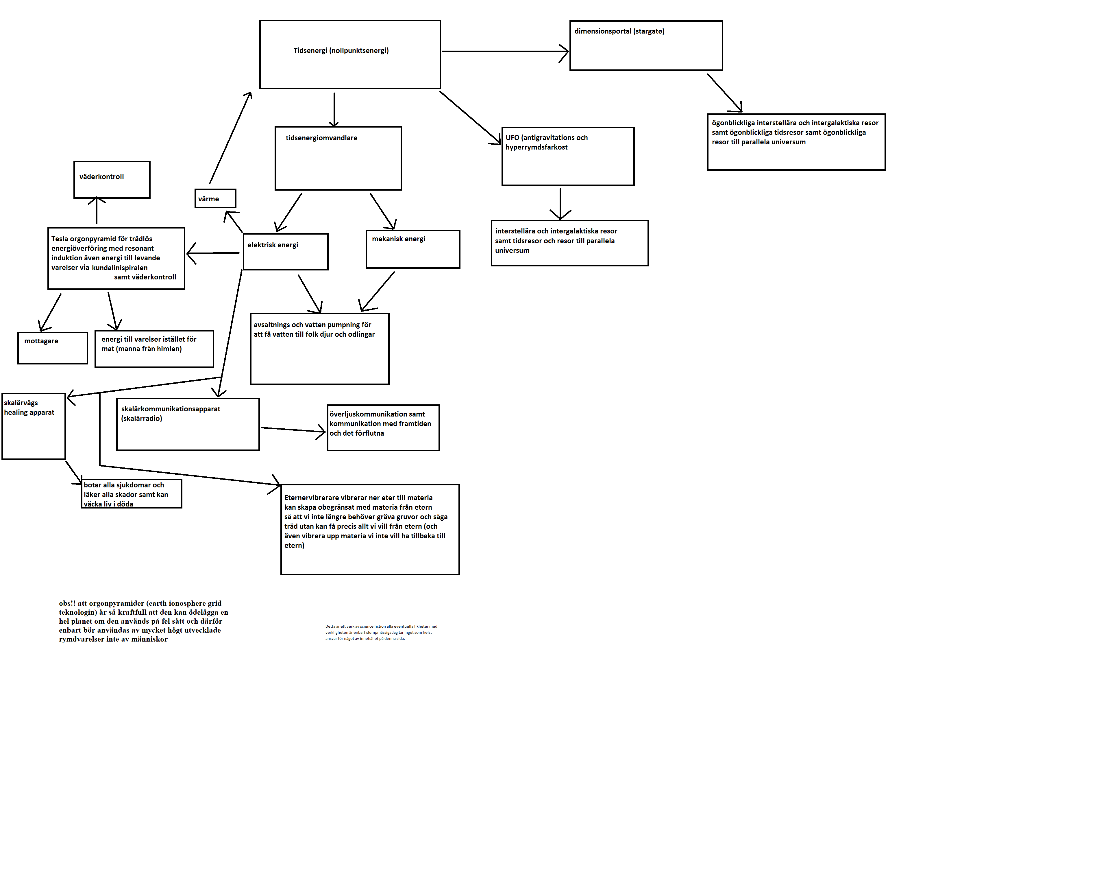