Blogg :: heliga tidsdimensionen

Blogg

A Pure Java HPCC Grid Architecture

01.05.2014 19:30

JUST.GridIACFeb2004.pdf (3,7 MB)

and CLE, Department of High Performance Computing

LOGISTIK ZENTRUM

CLE

JUSTGrid

A Pure Java HPCC Grid Architecture

for Multi-Physics Solvers

Using Complex Geometries.

Jochem Hauser*, Thorsten Ludewig*

Torsten Gollnick*, and Hans-Georg Paap†

*Dept. of High Performance Computing

Center of Logistics and Expert Systems (CLE) GmbH

Salzgitter, Germany

†HPC Consultant

Barbing, Germany

presented at

IAC Rome, Italy, 2 February 2004

Jochem Hauser et al. IAC Rome, Italy, 2 February 2004

Overview

Why Java for HPCC?!

What is JUSTGrid? (Framework)

JUSTGrid Communication Overview

Object Oriented Programming (OOP)

Threads

Graphical Applications

Java Performance Results

Conclusions

Future Work

Jochem Hauser et al. IAC Rome, Italy, 2 February 2004

Java as the Language for HPCC

platform independence

simple and straight forward parallelization

unique included network capabilities

JDBC (Java Database Connectivity)

RMI (Remote Method Invocation)

Secure Connections over the Inter- and Intranet

easy generation of object reflecting the engineering design

process

,,code reusability'' - simplifies code design

Jochem Hauser et al. IAC Rome, Italy, 2 February 2004

Why we like to use Java for writing highquality

portable parallel programs?

pure object formulation (i.e. an object representation of a

wing, fuselage, engine etc. described by a set of classes

containing the data structures and methods for a specific

item)

strong typing

exception model

elegant threading

portability

Jochem Hauser et al. IAC Rome, Italy, 2 February 2004

What is JUSTGrid

This is an age of possibility, and IT is the driving force behind this

change that occurs on a global range.

High Performance Computing and Communications (HPCC) on a

global scale is the key of this new economy.

The need for accurate 3D simulation in numerous areas of

computationally intensive industrial applications, including the rapidly

evolving field of bioscience, requires the development of ever more

powerful HPCC resources for a computational Grid based on the

Internet.

Jochem Hauser et al. IAC Rome, Italy, 2 February 2004

What is JUSTGrid

The Java language has the potential to bring about a revolution in

computer simulation. Using Java's unique features, a multidisciplinary

computational Grid, termed JUSTGrid, can be built

entirely in Java in a transparent, object-oriented approach.

JUSTGrid provides the numerical, geometric, parallel, and network

infrastructure for a wide range of applications in 3D computer

simulation thus substantially alleviating the complex task of software

engineering.

Jochem Hauser et al. IAC Rome, Italy, 2 February 2004

Scope of JUSTGrid

3D Complex Geometries

Parallelization

Dynamic Load Balancing

Internet

Collaborative

Engineering Outsourcing Interactive

Steering

System

Security

Solver Visualization

Navier Stokes

(fluid dynamics)

Maxwell

(electromagnetics)

Schrödinger

(quantum mechanics)

Surface

Conversion

Debugging

Results Session Tracking

JUSTGrid a framework for HPCC in engineering,

science, and life sciences

Jochem Hauser et al. IAC Rome, Italy, 2 February 2004

Scope of JUSTGrid

A solver only needs to contain the physics and numerics

of the simulation task for a single block or a single

domain.

The solver does not need to know anything about the

geometry data or the parallelization.

It has a simple structure

The solver can be tested independently before its

integration

Replacing the default solver by one's own solver.

Jochem Hauser et al. IAC Rome, Italy, 2 February 2004

Communication Overview

RMI based

Network

Solver/Code Development

Visualization

Collaborative Engineering

Server

Session-ID

Jochem Hauser et al. IAC Rome, Italy, 2 February 2004

Communication Overview

Client Server

Client

sends the data AND the java solver code to the

server and receives a unique session id to

identify the session on the server.

Server

provides a framework for multi physics solver

Database Server

interactive steering

Jochem Hauser et al. IAC Rome, Italy, 2 February 2004

Communication Overview

Client Server

with the unique session id everyone can

connect to a specific session on the server

start / stop session

changing the conditions of the computation

visualization

debugging

collaborative work

Jochem Hauser et al. IAC Rome, Italy, 2 February 2004

OOP - Object Oriented

Programming

Abstract Data Types

The association between the declaration of a data type and

the declaration of the code that is intended to operate upon

variables of this type

Data hiding and encapsulation

Protecting the data of an object from improper modification

by forcing the user to access the data trough a method.

class name

+variable1: integer

+variable2: double

+method1

+method2

Encapsulation of

data in an Object

Jochem Hauser et al. IAC Rome, Italy, 2 February 2004

OOP Example

Programming in 'C'

Programming in 'Java'

struct my_date {

int day, month, year;

} date;

date.day = 32;

public class MyDate {

private int day, month, year;

public void setDay( int day ) {

... validation code ...

}

MyDate myDate = new MyDate();

myDate.setDay( 32 );

ERROR!

Jochem Hauser et al. IAC Rome, Italy, 2 February 2004

Threads

an efficient way of parallelizing codes

What are Threads?

Multithreaded programs extends the idea of multitasking by

taking it one level further: individual programs (processes) will

appear to do multiple tasks at the same time.

Programs that can run more than one thread at once are said

to be multithreaded.

Each task is usually called thread which is the short form for

thread of control.

Jochem Hauser et al. IAC Rome, Italy, 2 February 2004

What are threads?

Three Parts of a Thread

A virtual CPU

The code the CPU is executing

The data the code works on

CPU

Code Data

A thread or

execution context

Jochem Hauser et al. IAC Rome, Italy, 2 February 2004

Why Threads are good for CFD

Threads as a general parallelization strategy for CFD

codes

Sophisticated dynamic load balancing algorithms on

shared-memory machines

Advanced numerical schemes in CFD, i.e. GMRES, do not

require the same computational work for each grid cell.

Jochem Hauser et al. IAC Rome, Italy, 2 February 2004

ClientGUI

Why we like to use simple graphical user interface for the

JUSTGrid?

Because for a non-Programmer it is to difficult to collect all

different parts needed for a JUSTGrid session into a Java

source text and compile it for himself.

It is easier to run a quick test case without falling into

common programming traps.

Jochem Hauser et al. IAC Rome, Italy, 2 February 2004

JUSTGrid Simple Client GUI

Jochem Hauser et al. IAC Rome, Italy, 2 February 2004

GRX Tool

Online

Visualization

Interactive

steering

Jochem Hauser et al. IAC Rome, Italy, 2 February 2004

GRX Tool

Online video generation

Integrated video player

Jochem Hauser et al. IAC Rome, Italy, 2 February 2004

GRX 3D Tool

Jochem Hauser et al. IAC Rome, Italy, 2 February 2004

Virtual Visualization Toolkit

(VVT / ShowMe3D)

The idea of ShowMe3D is to develop a light weight

application, which is easy to use, with a limited (but useful)

set of functionality.

visualization

Geometry (surface)

results of a computation

debugging

online client - server connection

e.g. boundary updates

surface converting

e.g. quads to triangles

Jochem Hauser et al. IAC Rome, Italy, 2 February 2004

ShowMe3D: Motivation

This program is designed for all programmers of Solver

Objects.

Based on the online "view" into the Server it can be very

helpful for debugging.

it is NOT designed to provide complete post processing

like TecPlot or Ensight

Jochem Hauser et al. IAC Rome, Italy, 2 February 2004

ShowMe3D (continued)

Today's implementation of ShowMe3D contains

Visualization

Geometry data

a tree view of the Java 3D scene graph

Surface conversion

for Alias Wave Front Objects only

Jochem Hauser et al. IAC Rome, Italy, 2 February 2004

ShowMe3D: main

The main window contains all the GUI elements for the file

input / output and visualization options

load geometry

save geometry

shaded view

wire frame view

system properties

Jochem Hauser et al. IAC Rome, Italy, 2 February 2004

ShowMe3D: file types

ShowMe3D can load 2D and 3D object data in different file

formats

Triangle

Plot3D

Plane 2D

Plane 3D

Volume 3D

Autodesk/AutoCAD DXF

AliasWavefront Objects

3D StudioMAX

LightWave

Jochem Hauser et al. IAC Rome, Italy, 2 February 2004

ShowMe3D: Application

Jochem Hauser et al. IAC Rome, Italy, 2 February 2004

Java High Performance and

Communications Test Suite

In the following series of slides we will demonstrate Java's

amazing numerical performance gains obtained over the

last few years.

Java numerical performance now rivals or exceeds that of

C or C++ codes used in engineering.

Jochem Hauser et al. IAC Rome, Italy, 2 February 2004

Simple numeric Benchmark

Simple numeric benchmark on a Sun Microsystems

Enterprise 10000 with 64 UltraSPARC II CPUs

1 2 3 4 5 6 7 8 910

36 37

500

1000

1500

2000

2500

3000

3500

4000

4500

5000

5500

6000

6500

7000

7500

8000

8500

9000

Simple numeric without communication 10e11 iterations

Time in s

Speedup

Number of CPUs

Time in seconds

Jochem Hauser et al. IAC Rome, Italy, 2 February 2004

Mandelbrot Benchmark

Mandelbrot Set dimension 7200 x 4800, max iterations

5000 running 400 threads on a Sun Microsystems

Enterprise 6000 with 28 processors.

This code tests the self-scheduling of threads.

1 2 3 4 5 6 7 8 9 10 11 12 13 14 15 16 17 18 19 20 21 22 23 24 25 26

0,0

2,5

5,0

7,5

10,0

12,5

15,0

17,5

20,0

22,5

25,0

27,5

10%

20%

30%

40%

50%

60%

70%

80%

90%

100%

110%

speedup

efficiency

Number of CPUs

Speedup

DEMO

Jochem Hauser et al. IAC Rome, Italy, 2 February 2004

Matrix Multiply

for comparison, we have a Java

and a C++-coded version of the

sequential block-matrix multiply

that does not use threads and

multithreaded Java and C++

version.

to compare floating point

performance for scientific

applications between C++ and

Java on the test machines

to measure parallel efficiency

of a multithreaded application

Exactly the following source was used

for both benchmarks. (C++ and Java)

// get start time here

for( n=0; n

{

for( i=0; i

{

for( j=0; j

{

for( k=0; k

{

c[i][j] += a[i][k]*b[k][j];

}

// get end time here

Jochem Hauser et al. IAC Rome, Italy, 2 February 2004

Sequential Matrix Multiplication

Runtime (2GHz Pentium 4, 1GB Memory) 1 run 2 run 3 run 4 run 5 run 6 run 7 run 8 run

3,15 3,19 3,22 3,16 3,15 3,17 3,16 3,16

3,23 3,23 3,25 3,23 3,23 3,23 3,23 3,25

3,86 3,88 3,90 3,90 3,90 3,90 3,89 3,90

3,55 3,51 2,12 2,12 2,12 2,12 2,13 2,12

GNU g++ -O3 -mcpu=pentium4

-march=pentium4 -Wall (Version 3.3.1)

Intel icc -O3 -mcpu=pentium4 -march=pentium4

(Version 8.0)

Sun Java HotSpot Client VM

(Version 1.4.2_02-b03)

Sun Java HotSpot Server VM

(Version 1.4.2_02-b03)

A sequential (1 thread) matrix multiplication using a 30

times 30 matrix doing 10000 iterations on a single

processor Pentium 4 PC running Linux.

After the two warmup phases in the Sun Java HotSpot

Server VM. This runtime is about 1.5 times faster then the

compiled C++ binary.

Due to a Linker error we could not use the -fast option

with the Intel compiler.

Jochem Hauser et al. IAC Rome, Italy, 2 February 2004

Multithreaded Matrix Multiplication

Multithreaded matrix multiplication using a 100 times 100

matrix doing 10000 iterations with 400 threads on a 26

CPU Sun Microsystems Enterprise 6000.

Runtime time in s

1.1.8_14 516,94

1.2.2_08 38,97

1.3.0_03 Server 37,47

1.3.1_02 Server 21,69

1.4.0_01 Server 19,51

1.4.1_02 Server 17,31

C++ - GCC 26,65

C++ - Forte 6u1 17,26

Jochem Hauser et al. IAC Rome, Italy, 2 February 2004

Multi-threaded Matrix Multiplication

Results a 100 x 100 matrix doing 10,000 iterations with 400

threads on the E6000 (26 CPUs)

1 2 3 4 5 6 7 8 9 10 11 12 13 14 15 16 17 18 19 20 21 22 23 24 25 26

0,0

2,5

5,0

7,5

10,0

12,5

15,0

17,5

20,0

22,5

25,0

10%

20%

30%

40%

50%

60%

70%

80%

90%

100%

110%

speedup

efficiency

Number of CPUs

Speedup

Jochem Hauser et al. IAC Rome, Italy, 2 February 2004

Euler 3D Comparison

As a reference sample to check the correct

communication (boundary update) of the JUSTGrid we

computed a 3D cone with the JUST Euler 3D solver and

CFD++

JUST Euler 3D

CFD++

Jochem Hauser et al. IAC Rome, Italy, 2 February 2004

Conclusions

With JUSTGrid a modern, well structured, easy to use and extensible

framework for HPCC is provided.

The code developer is freed from dealing with complex geometries, dynamic

load balancing and inter block or domain communication.

A numerical framework for a system of hyperbolic conservation laws is

installed, based on the integral form of the conservation equations

The parallel efficiency is obtained if a sufficient number of threads and

sufficient computational work within a thread can be provided.

The execution speed of Java code has increased substantially over the last few

years and now rivals the speed of C and C++ codes. More is too be expected.

Further work will be needed, but we following Kernighan's rules Make it right

before you make it faster as well as Don't patch bad code, rewrite it, the latter

rule being the reason for a pure Java flow solver code.

Jochem Hauser et al. IAC Rome, Italy, 2 February 2004

Future Work

Extending the JUSTGrid parallel layer to work with

distributed memory machines (Beowulf cluster). (e.g.,

JavaSpaces, JINI, Sockets)

Jochem Hauser et al. IAC Rome, Italy, 2 February 2004

Acknowledgments

This work is partly funded by the ministry of Sciences and

Culture of the State of Lower Saxony, Germany under

AGIP 1999.365 EXTV program.

We are particularly grateful to Sun Microsystems,

Benchmark Center, Germany for providing exclusive

access to a 28 CPU Sun Enterprise 6000 server.

We are grateful to Mr. Jean Muylaert for providing

information about the European eXperimental Test

Vehicle.

This work is part of the Ph.D. work of Thorsten Ludewig

Jochem Hauser et al. IAC Rome, Italy, 2 February 2004

References

Ginsberg,M., Häuser,J.,Moreira, J.E.,Morgan R., Parsons, J.C., Wielenga, T.J.

Panel Session: future directions and challenges for Java implementations of numeric-intensive industrial

applications published in: Advances in Engineering Software, Elsevier, 31,2000, p.743-751

Häuser,J., Ludewig, T., Williams, Roy D., Winkelmann, R., Gollnick, T., Brunett, S., Muylaert, J.

A Test Suite for High Performance Parallel Java published in: Advances in Engineering Software, Elsevier,31,

2000, p.687-696

Häuser,J., Ludewig, T., Williams, Roy D., Winkelmann, R., Gollnick, T., Brunett, S., Muylaert, J.

A Test Suite for High Performance Parallel Java paper presented at 5th National Symposium on Large-Scale

Analysis, Design and Intelligent Synthesis Environments, Williamsburg, VA, October 12th to 15th, 1999

Häuser,J., Ludewig, T., Williams, Roy D., Winkelmann, R., Gollnick, T., Brunett, S., Muylaert, J.

NASA Panel Java Soundbytes paper presented at 5th National Symposium on Large-Scale Analysis, Design and

Intelligent Synthesis Environments, Williamsburg, VA, October 12th to 15th, 1999

Häuser, J., Ludewig, Th., Gollnick, T., Winkelmann, R., Williams, R., D., Muylaert, J., Spel, M.,

A Pure Java Parallel Flow Solver, published in: Proceedings of the 37th AIAA Aerospace Sciences Meeting and

Exhibit, AIAA 99-0549 Reno, NV, USA, January 11.-14., 1999.

Häuser J., Williams R.D, Spel M., Muylaert J., ParNSS: An Efficient Parallel Navier-Stokes Solver for Complex

Geometries, AIAA 94-2263, AIAA 25th Fluid Dynamics Conference, Colorado Springs, June 1994.

JUST.GridIACFeb2004.pdf (3,7 MB)

Current Research in Gravito-Electromagnetic Space Propulsion

01.05.2014 19:18

LauncherSymPaper2007-0-42.pdf (4,6 MB)

Current Research in Gravito-Electromagnetic

Space Propulsion

Walter Dröscher and Jochem Hauser 1

Institut für Grenzgebiete der Wissenschaft, 6010 Innsbruck, Austria

Abbreviated Version 2

Figure 1. The figure shows a combination of two pictures. The first one shows an artist’s concept of two Jupiter like planets,

detected by NASA’s Spitzer Space Telescope. Spitzer captured for the first time, February 2007, enough light to take the spectra

of these two gas exoplanets, called HD 209458b and HD 189733b. These so-called "hot Jupiters" are like Jupiter, but orbit much

closer to their sun. Molecules were identified in their atmospheres. HD 189733b is about 63 light years away in the constellation

Vulpecula, and HD 209458b is approximately 153 light years away in the constellation Pegasus. The second picture, lower right,

depicts the principle of gravito-magnetic space propulsion. For further explanations see Fig. 5 of this paper.

1 Permanent address: Faculty Karl-Scharfenberg, Univ. of Applied Sciences, Salzgitter Campus, 38229 Salzgitter, Germany

2 Mathematical derivations were omitted in this abbreviated version

3 4 5

Abstract: Spaceflight, as we know it, is based on the century old rocket equation that is an embodiment of the conservation of

linear momentum. Moreover, special relativity puts an upper limit on the speed of any space-vehicle in the form of the velocity

of light in vacuum. Thus current physics puts severe limits on space propulsion technology.

This paper presents both recent theoretical and experimental results in the novel area of propulsion research termed gravitomagnetic

field propulsion comprising the generation of artificial gravitational fields. In the past, experiments related to any

kind of gravity shielding or gravito-magnetic interaction proved to be incorrect. However, in March 2006 the European Space

Agency (ESA) announced credible experimental results, reporting on the measurement of artificial gravitational fields (termed

gravito-magnetic fields), generated by a rotating Niobium superconductor ring that was subjected to angular acceleration. These

experiments were performed by M. Tajmar and colleagues from ARC Seibersdorf, Austria and C. de Matos from ESA, and

recently were repeated with increased accuracy.

Extended Heim Theory (EHT), published in a series of papers since 2002, predicted the existence of such an effect, resulting

from a proposed interaction between electromagnetism and gravitation. In EHT, which is a consequent extension of Einstein’s

idea of geometrization of all physical interactions, the concept of poly-metric developed by the German physicist B. Heim

is employed. As a consequence of this geometrization, EHT predicts the existence of six fundamental interactions. The two

additional interactions are identified as gravitophoton interaction, enabling the conversion of photons into a gravitational

like field, represented by two hypothetical gravitophoton (attractive and repulsive) particles, and the quintessence particle,

a weak repulsive gravitational like interaction (dark energy?). The experiments by Tajmar et al. (the artificial gravitational

force, however, was observed only in the circumferential direction of the superconducting ring) can be explained by the joint

generation of quintessence particles and gravitons. EHT is used to provide a physical model for the existence of the artificial

gravitational field, and to perform comparisons with experimental data.

In the next step, it is shown that the gravitophoton interaction could be used to devise a novel experiment in which the artificial

gravitational field would be directed along the axis of rotation, and thus this force could serve as the basis for a field propulsion

principle working without fuel. Based on this novel propulsion concept, missions to the international space station (LEO), the

planned moon basis, to Mars, and missions to the outer planets are analyzed. Estimates for the magnitude of magnetic fields

and necessary power are presented as well as for trip times.

PRESENT CONCEPTS OF SPACE PROPULSION

Current space transportation systems are based on the principle of momentum generation, regardless whether they

are chemical, electric, plasma-dynamic, nuclear (fission) or fusion, antimatter, photonic propulsion (relativistic)

and photon driven (solar) sails, or exotic Bussard fusion ramjets. The specific impulse achievable from thermal

systems ranges from some 500 s for advanced chemical propellants (excluding free radicals or metastable atoms),

approximately 1,000 s for a fission solid-core rocket (NERVA program [1] ) using hydrogen as propellant (for a

gas-core nuclear rocket specific impulse could be 3,000 s or higher but requiring very high pressures), and up to

200,000 s for a fusion rocket [2]. Although recently progress was reported in the design of nuclear reactors for plasma

propulsion systems [3] such a multimegawatt reactor has a mass of some 3106 kg and, despite high specific impulse,

has a low thrust to mass ratio, and thus is most likely not capable of lifting a vehicle from the surface of the earth.

For fusion propulsion, the gasdynamic mirror has been proposed as highly efficient fusion rocket engine. However,

recent experiments revealed magnetohydrodynamic instabilities [4] that make such a system questionable even from a

physics standpoint, since magnetohydrodynamic stability has been the key issue in fusion for decades. The momentum

principle combined with the usage of fuel, because of its inherent physical limitations, does not permit spaceflight to

be carried out as a matter of routine without substantial technical expenditure.

At relativistic speeds, Lorentz transformation replaces Galilei transformation where the rest mass of the propellant

is multiplied by the factor (1=

1¤v2=c2) that goes to infinity if the exhaust velocity v equals c, the speed of light in

vacuum. For instance, a flight to the nearest star at a velocity of some 16 km/s would take about 80,000 years. On the

other hand, a space vehicle with a mass of 106 kg at the high velocity of 105 km/s would take approximately 12.8 years

to reach this star. Its kinetic energy would amount to about 51021 J. Supplied with a 100 MW nuclear reactor, it

would take some 1.5 million years to generate this amount of energy. Current physics requires that energy conservation

is strictly adhered to and does not permit to extract energy from the vacuum. However the physical properties of the

3 Invited paper O-42, plenary session 7th International Symposium on Launcher Technologies 2007, 2-5 April 2007, Barcelona, Spain

4 ©Institut für Grenzgebiete der Wissenschaft Innsbruck, Austria 2007

5 The mathematical derivations in this paper rely on concepts explained in paper [11]. For lack of space these concepts are not presented here, see

www.hpcc-space.de for download.

vacuum are not known [18]. The energy density of the vacuum calculated by General Relativity (GR) and Quantum

Field Theory (QFT) differ by a factor of 10108, which means the error is in the exponent. Current physics clearly is open

to question. Moreover, it is obvious that if the speed of light cannot be transcended, interstellar travel is impossible.

We conclude with a phrase from the recent book on future propulsion by Czysz and Bruno [19]: If that remains the

case, we are trapped within the environs of our Solar System. In other words, the technology of spaceflight needs to be

based on novel physics that provides a novel propulsion principle. Most likely the physical properties of the vacuum

play an important role, although unknown at present.

Although advanced propulsion concepts as the ones described above must be pursued further, a research program

to look for fundamentally different propulsion principles is also both needed and justified, especially in the light of the

recent experiments by Tajmar et al. concerning the measurements of artificial gravitational fields [5], [6], [7], [8]. For

a popular description of this experimental work see [9], [10].

In addition, since 2002 ideas for a fundamental physical theory, termed Extended Heim Theory (EHT), predicting

two additional physical interactions that might give rise to the generation of artificial gravitational fields, have been

published, see for instance, [11], [12], [13], [14]. A popular description of this research may be found in [15], [16],

[17]. In the subsequent sections, EHT will be used to reproduce experimental values measured by Tajmar et al. and to

provide guidelines for a novel experiment that would serve as demonstrator for a propellantless propulsion device.

Needless to say, these ideas are highly speculative and their correctness can only be proved by experiment. However,

EHT makes precise predictions about the type and number of possible physical interactions. The proposed experiment

can be carried out with current technology to verify theoretical predictions.

PHYSICAL INTERACTIONS AND GEOMETRIZATION

In this section the fundamental structure of spacetime is discussed. The main idea of EHT is that spacetime possesses

an additional internal structure, described by an internal symmetry space, dubbed Heim space, denoted H8, which

is attached to each point of the spacetime manifold. The internal coordinates of H8 depend on the local (curvilinear)

coordinates of spacetime. This is analogous to gauge theory in that a local or gauge transformation is used. In gauge

theory it is the particles themselves that are given additional degrees of freedom, expressed by an internal space.

Consequently in the geometrization of physics, it is spacetime instead of elementary particles that has to be provided

with internal degrees of freedom. The introduction of an internal space has major physical consequences. The structure

of H8 determines the number and type of physical interactions and subsequently leads to a poly-metric. This means that

spacetime comprises both an external and internal structure. In general, only the external structure is observed,

but as has long been known experimentally, matter can be generated out of the vacuum. This is a clear sign that

spacetime has additional and surprising physical properties. Therefore, any physical theory that aims at describing

physical reality, needs to account for this fact. Since GR uses pure spacetime only, as a consequence, only part of the

physical world is visible in the form of gravitation.

This idea was first conceived by the German physicist B. Heim. A similar principle was mentioned by the Italian

mathematician B. Finzi. The poly-metric tensor resulting from this concept is subdivided into a set of sub-tensors, and

each element of this set is equivalent to a physical interaction or particle, and thus the complete geometrization of

physics is achieved. This is, in a nutshell, the strategy chosen to accomplish Einstein’s lifelong goal of geometrization

of physics 6. It must be noted that this approach is in stark contrast to elementary particle physics, in which particles

possess an existence of their own and spacetime is just a background staffage [32]. In EHT, considered as the

natural extension of GR, matter simply is a consequence of the hidden physical features of spacetime. These two

physical pictures are mutually exclusive, and experiment will show which view ultimately reflects physical reality. It

is, however, well understood that the concept of a pointlike elementary particle is highly useful as a working hypothesis

in particle physics.

6 There is of course a second aspect, namely the quantization of the spacetime field.

Geometrization of Space, Time, and Energy

In GR the geometrical structure of spacetime leads to a single metric that describes gravitational interaction.

Einstein’s pioneering efforts in the geometrization of physics revealed themselves unsuccessful [22] when more

interactions were discovered, and attempts to geometrize physics were abandoned. Einstein did not succeed in

constructing a metric tensor that encompassed all physical interactions. At almost the same time, B. Heim at the

space congress in Stuttgart, Germany 1952 and in [23], and also B. Finzi, 1955, see the recent book [24], published

similar ideas on the construction of a generalized metric tensor. Heim published further details of his theory in [25],

[26] constructing a poly-metric tensor in a 6D space. In collaboration with Heim this idea was extended to 8D by the

first author.

Einsteinian spacetime [20], [21] is indefinitely divisible and can be described by a differentiable manifold. In the

following derivation, which relates the metric tensor to physical interactions, this classical picture is used, though

most likely spacetime is a quantized field. The quantization of spacetime seems to play a role in the concept of

hyperspace or parallel space [14], which might allow superluminal velocities, but is not treated in this paper. GR can

be summarized by the single sentence: matter curves spacetime.

In curved spacetime the metric is written in the form

ds2 = gmndhmdhn (1)

where gmn is the metric tensor, h1;h2;h3 are the spatial coordinates, and h4 is the time coordinate. These coordinates

can be curvilinear. Einstein summation convention is used, i.e., indices occurring twice are summed over. From the

strong equivalence principle it is known (for instance see [27]) that at any point in spacetime a local reference frame

can be found for which the metric tensor can be made diagonal, i.e., gmn = hmn where hmn is the Minkowski tensor, 7

and reference coordinates are locally Cartesian (x1; x2; x3; x4) = (x; y; z; ct). This is equivalent to a transformation

between the two sets of coordinates, namely

dxm = Lm

n dhn and Lm

n =

¶ xm

¶hn (2)

In the free fall frame of the x coordinates the acceleration is 0, and thus the equation of motion simply is

d2xm

dt2 = 0 and ds2 = hmn dxmdxn (3)

where t denotes proper time, i.e., the time registered by a clock in its own reference frame. This means the clock is

stationary in this frame, and the time measured is the time shown on the clock’s dial. In order to obtain the equation of

motion for curvilinear coordinates h, one only needs to insert the transformation relations, Eq. (2), into Eq. (3), which

results in the geodesic equation

d2ha

dt2 +Gamn

dhm

dhn

= 0 (4)

where the Gam

n are the well known Christoffel symbols or affine connections. Rewriting the geodesic equation (4) in

the form

d2ha

dt2 = f a with f a = ¤Gam

dhm

dhn

dt (5)

and comparing Eq. (5) with the equation of motion for a free falling particle Eq. (3), the right hand side of Eq. (5)

can be regarded as a force coming from a physical interaction, which has caused a curvature of the surrounding space,

marked by the presence of nonzero Christoffel symbols. The left hand side of equation (5) can be written as mIa where

mI denotes inertial mass and a is acceleration. Multiplying f a by its proper charge results in the equation of motion

for the respective physical interaction. In the case of gravity, because of the equality of inertial and gravitational mass,

charges on the left and right hand sides cancel out. For all other physical interactions this is not the case. In that respect

7 Minkowski tensor hmn must not be confused with curvilinear coordinates hm

gravity has a unique role, namely that it curves also the surrounding space. For all other physical interactions, if

pointlike charges are assumed (classical picture), space is curved only at the location of the charge.

One major point of course is that the relation x = x(h) as used in GR delivers only a single metric, which

Einstein associated with gravitation. The fundamental question is, therefore, how to construct a metric tensor that

gives rise to all physical interactions. The answer lies in the fact that in EHT there exists an internal space H8.

Therefore, in EHT the relation between coordinates x and h is x = x(x (h)). In contrast to GR, EHT employs a

double transformation as specified in Eq. (7). From this double transformation a set of different metric tensors can

be constructed, which, in turn, lead to a set of individual geodesic equations having the same structure as Eq. (5), but

depending on the specific charge and Christoffel symbols inherent to this specific physical interaction. An individual

equation of motion will have the form

d2hm

dt2 = ec f m

c with m = 1; :::;4 (6)

where ec denotes the specific charge of the interaction and quantities f m

c are the associated Christoffel symbols 8

i.e., they stand for the curvature of space generated by this interaction. The total number of physical charges ec is

determined by the subspace structure of H8 in concert with combination rules to constructing a metric that has physical

meaning. Eq. (6) describes a very difficult physical problem. First, the number of physical charges and their coupling

constants need to be determined. Without further demonstration, only a few facts are stated. There exist, according

to EHT, eight charges, namely three color charges for the quarks, two weak charges, one electric charge, and two

charges for gravitation, where one naturally is the gravitational charge. The second charge could be inertia or the

charge of the vacuum. This is not clear at present. The double transformation as given in Eq. (7) represents the particle

aspect and leads to eigenvalue equations whose eigenvalues have dimension of inverse length. In these eigenvalue

equations, the Christoffel symbols occur. Using the inverse of the Planck length expressed as mpc=¯h, results in a

correspondence between inverse length and mass. Since particles and fields form a unity, the transformation from

spacetime into internal space, M !H8, should represent the field aspect, because derivatives of internal coordinates

x a;a = 1; :::;8 with respect to curvilinear coordinates h lead to an expression

ik. The ha

ik denote deviation from

the flat metric, and physically represent the tensor potential of the charge ea

c with mI as associated inertial mass.

The metric coefficients thus assume energy character. This short discussion implies a comprehensive mathematical

program, namely the determination and solution of the above mentioned eigenvalue equations as well as the derivation

of the tensor potentials for the interactions. The task is not yet finished, but this brief discussion should have conveyed

an idea how the introduction of an internal symmetry space leads to a correspondence between geometry and physical

quantities. 9 10

This approach is substantially different from GR and leads to the complete geometrization of physical

interactions.

Naturally, the number and type of interactions depend on the structure of internal space H8 whose subspace

composition is determined in the subsequent section. Contrary to the ideas employed in String theory, see for example

[28], H8 is an internal space of 8 dimensions that, however, governs all physical events in our spacetime.

The crucial point lies in the construction of the internal space whose subspace composition should come from basic

physical assumptions, which must be generally acceptable. In other words, GR does not possess any internal structure,

and thus has a very limited geometrical structure, namely that of pure spacetime only. Because of this limitation, GR

cannot describe other physical interactions than gravity, and consequently needs to be extended. EHT in its present

form without any quantization, i.e., not using a discrete spacetime, reduces to GR when this internal space is omitted.

The metric tensor, as used in GR, has purely geometrical means that is, it is of immaterial character only, and does

not represent any physics. Consequently, the Einsteinian Geometrization Principle (EGP) is equating the Einstein

curvature tensor, constructed from the metric tensor, with the stress tensor, representing energy distribution. In this

way, the metric tensor field has become a physical object whose behavior is governed by an action principle, like that

8 The equation of motion describes a particle of mass mI with charge ec, subjected to the respective field of this interaction, represented by its

proper Christoffel symbols.

9 The mathematical framework to determine the charges and to obtain the correspondence between geometry and physics is quite involved. In

general internal coordinates are described by quaternions.

10 There is an interesting question, namely: What is the Hermetry form of the vacuum field ? If the vacuum has an energy density different from

zero, it should not be the case that its Christoffel symbols are 0. However, we feel, in order to answer this question, a quantization procedure for Eq.

(6) has to be established.

of other physical entities. In EHT the internal space H8 is associated with physics through the introduction of three

fundamental length scales, constructed from Planck quantities.

FUNDAMENTAL INTERACTIONS AND HERMETRY FORMS

The introduction of basic physical units is in contradiction to classical physics that allows infinite divisibility. As a

consequence, measurements in classical physics are impossible, since units cannot be defined. Consequently, Nature

could not provide any elemental building blocks to construct higher organized structures, which is inconsistent with

observation. Thus the quantization principle is fundamental for the existence of physical objects.

Next, we introduce four basic principles, from which the nature of H8 can be discovered. In contrast to GR, EHT is

based on the following four simple and general principles, termed the GODQ principle 11 of Nature. These principles

cannot be proved mathematically, but their formulation is based on generally accepted observations and intend to

reflect the workings of Nature.

i. Geometrization principle for all physical interactions,

ii. Optimization (Nature employs an extremum principle),

iii. Dualization (duality, symmetry) principle (Nature dualizes or is asymmetric, bits),

iv. Quantization principle (Nature uses integers only, discrete quantities).

From the duality principle, the existence of additional internal symmetries in Nature is deduced, and thus a higher

dimensional internal symmetry space should exist, whose exact structure will now be determined. In GR there exists a

four dimensional spacetime, comprising three spatial coordinates with positive signature (+) and the time coordinate

with negative signature (-). It should be remembered that the Lorentzian metric of R4 has three spatial (+ signature)

and one time-like coordinate (- signature) 12. The corresponding metric is called Minkowski metric and the spacetime

associated with this metric is the Minkowski space. The plus and minus signs refer to the (local) Minkowski metric

(diagonal metric tensor, see Eq. (1). Therefore, the squared proper time interval is taken to be positive if the separation

of two events is less than their spatial distance divided by c2. A general coordinate system for a spacetime manifold,

M, needs to be described by curvilinear coordinates hm with m = 1; ::;4 and h = (hm ) 2 M.

The set of 8 internal coordinates for H8 is determined by utilizing the GODQ principle. There are three internal

spatial coordinates, x 1;x 2;x 3, and the internal time coordinate x 4. The other four coordinates are introduced to

describing the degree of organization and information exchange as observed in Nature.

In summary, internal coordinates x i with i=1; :::;4 denote spatial and temporal coordinates, x i with i=5;6 denote

entelechial and aeonic coordinates, and x i with i = 7;8 denote the two information coordinates in H8, mandating

four different types of coordinates. With the introduction of a set of four different types of coordinates, the space

of fundamental symmetries of internal space H8 is fixed. In the next section, the set of metric subtensors of H8 is

constructed, each of them describing a physical interaction or particle. Thus the connection between physical space

and physics (symmetries) is established in a way foreseen by Einstein. Physical space is responsible for all physical

interactions. However, in order to reach this objective, spacetime had to be complemented by an internal space H8 to

model its physical properties. Once the internal space with its set of coordinates has been determined, everything else

is fixed, because Eq. (7) is a direct consequence of H8 .

It should be noted that a dimensional law can be derived that does not permit the construction of, for instance,

a space H7 [26]. In order to determine the number of admissible Hermetry forms and their physical meaning, we

proceed as follows. As was shown above, Heim space, H8, comprises four subspaces, denoted as R3 with coordinates

x 1;x 2;x 3, T1 with coordinate x 4, S2 with coordinates x 5;x 6 , and I2 with coordinates x 7;x 8: In order to construct a

physically meaningful metric sub-tensor (also called Hermetry form), it is postulated that coordinates of internal

spaces S2 or I2 must be present in any metric subtensor to generate a Hermetry form. From this kind of selection rule,

it is straightforward to show that 12 Hermetry forms can be generated, having direct physical meaning. In addition,

there are three degenerated Hermetry forms that describe partial forms of the photon and the quintessence potential,

11 briefly stated: God quantizes.

12 Signatures are not unique. Coordinate signatures may be reversed. Numbering of coordinates was chosen such that coordinates of positive

signature are numbered first.

for details see Tables 2, 4 of ref. [11]13. Hermetry form 16 is reserved for the Higgs particle that should exist, whose

mass was calculated at 182:70:7 GeV. For instance, the Hermetry form (photon metric) comprises only coordinates

from subspaces T1 , S2 , and I2 and is denoted by H7(T1 S2 I2). The neutral gravitophoton Hermetry form is

given by H5(S2 I2). Since gravitophoton and photon Hermetry forms are described by different coordinates, they

lead to different Christoffel symbols, and thus to different geodesic equations, see Eq. (6). Furthermore, if there were

a physical process to eliminate the T1 coordinates, i.e., the corresponding Christoffel symbols are 0, the photon would

be converted into a gravitophoton. This is how mixing of particles is accomplished in EHT. We believe this to be

the case in the experiments by Tajmar et al. The fundamental question, naturally, is how to calculate the probability

of such a process, and to determine the experimental conditions under which it can take place. Hermetry forms alone

only provide the potential for conversion into other Hermetry forms, but nothing is said about physical realization.

In any case, if Hermetry forms describe physical interactions and elementary particles, a completely novel scenario

unfolds by regarding the relationships between corresponding Hermetry forms. Completely new technologies could be

developed converting Hermetry forms. In the section about the proposed gravito-magnetic field propulsion experiment,

an experiment utilizing a rotating disk is described to convert photons into positive (repulsive) and negative (attractive)

gravitophotons that should generate an artificial gravitational field along the axis of rotation.

Fig. (2) depicts the six fundamental forces predicted by EHT. From the neutral gravitophoton metric and from the

forces measured in the experiments, it is deduced that the gravitophoton decays into a graviton (H1) and a quintessence

(H9, repulsive) particle. Fig. (3) shows the set of metric-subspaces that can be constructed. The word Hermetry is a

combination of hermeneutics and geometry that is, a Hermetry form stands for the physical meaning of geometry.

Each Hermetry form has a direct physical meaning, for details see refs. [11], [13], [14].

Double Coordinate Transformation

In this section the mathematical details of constructing Hermetry forms are presented. The concept of an internal 8D

space, comprising four subspaces, leads to a modification of the general transformation being used in GR. In GR there

are two sets of coordinates, Cartesian coordinates x and curvilinear coordinates h linked by a relation between their

corresponding coordinate differentials, Eqs. (1, 2). If Heim space were not existing, the poly-metric of EHT collapsed

to the mono-metric of GR.

The existence of internal space H8 demands a more general coordinate transformation from a spacetime manifold

14 M to a manifold N via the mapping M (locally R4 ) ! H8 ! N (locally R4 ). In EHT, therefore, a double

transformation, Eq.(7), involving Heim space H8 occurs. The associated global metric tensor, Eq. (7), does not have

any physical meaning by itself. Instead, by deleting corresponding terms in the global metric, the proper Hermetry

form is eventually obtained. The global metric tensor is of the form

gik =

¶ xm

¶ x a

¶hi

¶ xm

¶ x b

¶hk (7)

where indices a;b = 1; :::;8 and i;m;k = 1; :::;4 and gik comprises 64 components. The tensor with all 64 terms

does not have a physical meaning.

A single component of the metric tensor belonging to one of the four subspaces is given by Eq. (8). Only special

combinations of the gab

ik reflect physical quantities. Because of the double transformation, each physically meaningful

metric does comprise a different subset of the 64 components. In other words, depending on the Hermetry form, a

specified number of components of the complete metric tensor in spacetime, Eq. ((7), are set to zero. Hence, each

Hermetry form is marked by the fact that only a subset of the 64 components is present. Therefore each Hermetry

form leads to a different metric in the spacetime manifold and thus describes different physics. This is why Eq. ((7)

is termed the poly-metric tensor. It serves as a repository for Hermetry forms. This construction principle is totally

different from Einstein’s approach, and only in the special case of vanishing space H8 , EHT reduces to GR.

gab

ik =

¶ xm

¶ x (a)

¶hi

¶ xm

¶ x (b)

¶hk (8)

13 Tables 1-4 of ref. [11] were omitted from this paper because of lack of space

14 in the concrete case of GR spacetime manifold M4 would be used

Figure 2. EHT predicts, as one of its most important consequences, two additional, gravitational like interactions and the existence

of two messenger particles, termed gravitophoton and quintessence. That is, there is a total of six fundamental physical interactions.

The name gravitophoton has been chosen because of the type of interaction, namely the transformation of the electromagnetic field

(photon) into the gravitational field (gravitophoton). The arrow between the gravitophoton and electromagnetic boxes indicates

the interaction between these messenger particles that is, photons can be transformed into gravitophotons. In the same way

the quintessence interaction can be generated from gravitons and positive gravitophotons (repulsive force). It is assumed that

first a neutral gravitophoton is generated that decays into a pair of negative (same sign as gravitational potential) and positive

gravitophotons.

The poly-metric tensor can be written as

gik =

8å

a;b=1

ga;b

ik (9)

A single Hermetry form is given by

gik(Hl) :=

8å

a;b2Hl

gab

ik (10)

It should be mentioned that each Hermetry form itself comprises a set of submetric tensors that are intrinsic to this

Hermetry form. In how far this is an indication for further substructures is not known at the moment. In any case, there

are three additional Hermetry forms that we denoted as degenerate Hermetry form. They are describing neutrinos

and two novel fields that were identified as conversion (probability) amplitudes wph_gp and wgp_q. The first amplitude

stands for the probability of converting photons into gravitophotons, the second one denotes the probability for a

gravitophoton to decay into a graviton and quintessence particle. These conversion equations play a major role in the

explanation of the experiments by Tajmar et al. as well as in the proposed field propulsion experiment.

Physical Meaning of Hermetry Forms

Here, we only can give a brief discussion of the meaning of Hermetry forms. Each of the 15 admissible combinations

(not counting the Higgs particle) of metric subtensors (Hermetry forms) is ascribed a physical meaning, see Tables 1-4

in ref. ([11]). A Hermetry form is denoted by Hl with l =1; :::;15 is used. Indices 1-12 are obtained from the definition

of the Hermetry forms, see Fig. (3). Each Hermetry form Hl is interpreted as physical interaction or particle, extending

the interpretation of metric employed in GR to the poly-metric, coming from the combination of external physical

spacetime and internal space that is, the interaction of space H8 with four-dimensional spacetime M4. Internal space

H8 is a factored space that is, it is represented as H8 = R3 T1 S2 I2. This factorization of H8 into one space-like

manifold R3 and three time-like manifolds T1, S2 and I2 is inherent to the structure of H8. Each subspace can be

associated with a symmetry group. H8 would be associated with group O(8), which in turn is also factored. For the

construction of the individual Hermetry forms, a selection rule is used, namely any physically meaningful Hermetry

form must contain space coordinates from S2 or I2. This means, for a physical process to become manifest in

spacetime, a pair of the transcoordinates (entelechial, aeonic or information coordinates) must occur in its metric, i.e.,

in its Hermetry form. Each individual Hermetry form is equivalent to a physical potential or a messenger particle. It

should be noted that a Hermetry form in space S2 I2 describes gravitophotons, and a Hermetry form constructed

from space S2 I2 T1 represents photons, see Table 2 in ref. ([11]). This is an indication that, at least on theoretical

arguments, photons can be converted into gravitophotons, if the time dependent part T1 of the photon metric can be

canceled. Fig. (3) shows the possible Hermetry forms in EHT.

Conversion Equations for Hermetry Forms

In the section above, the physical meaning of Hermetry forms was discussed. Regarding the Hermetry forms for the

photon, H7, and the gravitophoton, H5, see Table 2 in [11], it is straightforward to see that if all metric subcomponents

containing the time coordinate in the metric tensor of the photon are deleted, the metric of a neutral 15gravitophoton

is generated. The fundamental question is, of course, how this mathematical process can be realized as a physical

phenomenon.

Regarding further the Hermetry form of the neutral gravitophoton, it should be possible that under certain circumstances

this neutral gravitophoton becomes unstable and decays. According to its metric form, a neutral gravitophoton

can decay through two channels. In one case, a graviton and a quintessence particle can be generated. In the second

case, a positive (repulsive) and a negative (attractive) gravitophoton can be produced. The former seems to occur in

Tajmar’s experiments, see section below, and the latter case should happen in the proposed field propulsion experiment

outlined, see corresponding section.

A conversion of photons into gravitophotons should be possible in two ways, namely via Fermion coupling

according to Eqs. (12), (13) and through Boson coupling, described by Eqs. (14), (15). These equations are termed

conversion equations. The three conversion amplitudes have the following meaning: The first equation, Eq. (12) is

obtained from EHT in combination with considerations from number theory, and predicts the conversion of photons

into gravitophoton particles, published already in 1996 [35] while the second equation, Eq. (13), is taken from Landau

[36] where the probability amplitude wgp for the photon coupling is given by the well known relation

ph =

4pe0

¯hc

: (11)

The physical meaning of Eqs. (12), (13) lies in the production of N2 gravitophoton particles through the polarization

of the vacuum. This conversion process is termed Fermion coupling, because it is assumed that the production

of gravitophotons takes place at the location of a virtual electron. This process is described in detail in references [11],

[13], and [12]. As was further discussed in these references, the magnitude of the necessary magnetic induction, m0H,

15 a gravitophoton is termed neutral if it does not interact with matter

Figure 3. In EHT, each point in spacetime is associated with an internal Heim space H8 that has eight internal coordinates. These

coordinates are interpreted as energy coordinates. The Planck length lp is associated with spatial coordinates of space R3 , the

Planck length lt with the time coordinate of space T1 , and Planck length lmp with the four additional organization and information

coordinates (negative) signature, which give rise to two additional subspaces denoted as S2 and I2, respectively. Hence, Heim space

H8 comprises four subspaces, namely R3 , T1 , S2 , and I2. The 8 coordinates x n of H8 themselves are functions of the curvilinear

coordinates hm that is, x n = x n(hm) of physical spacetime, manifold M4. The picture shows the complete set of metric-subspaces

that can be constructed from the poly-metric tensor, Eq. (7). Each submetric is denoted as Hermetry form, which has a direct

physical meaning, see Table 2 in [11]. In order to construct a Hermetry form, either internal space S2 or I2 coordinates must be

present. In addition, there are three degenerated Hermetry forms, see Table 4 in [11] that are only partial metric forms of the photon

and the quintessence potential. They allow the conversion of photons into gravitophotons as well as the decay of gravitophotons

into gravitons and quintessence particles.

in order to obtain sufficient gravitophoton production to generate a sizeable gravitophoton force (or Heim-Lorentz

force), is in the range of 20 to 50 T, and thus is most likely beyond current technology.

wph(r)¤wph_gp = Nwgp (12)

wph(r)¤wph_gp = Awph (13)

Eq. (13) and the function A(r) can be obtained using Landau’s [36] radiation correction with numerical values for

A ranging from 10¤3to 10¤4. Eqs. (12) and (13) can be interpreted such that an electromagnetic potential (photon)

containing probability amplitude Awph can be converted into a neutral gravitophoton with associated probability

amplitude Nwgp. Landau’s equation, Eq. (13), is responsible for the additional charge, coming from the reduced

shielding of the vacuum.

When we analyzed the experiments by Tajmar et al. it became clear that there seems to be a second way to generate

a gravitophoton force, namely using Cooper pairs to trigger the production of neutral gravitophotons. Because of

the coupling through Cooper pairs, this conversion is dubbed Boson coupling, and is specified by Eqs.(14) and (15). It

turned out that the conversion of photons into gravitophotons through Boson coupling has substantially lower technical

requirements. Instead of changing the conversion amplitude wph(r) by reducing the distance between virtual electron

and proton below the Compton wavelength, lC, (for mathematical details see the above mentioned references), it is

now the value of the probability amplitude wph_gp that changes. In general, i.e., without the presence of Cooper pairs,

wph_gp = wph and, according to Eq. (15), the probability for gravitophoton production is 0. For the production process

to take place, it is assumed that the onset of superconducting - with its formation of Cooper pairs - has an effect

similar to the creation of electron-positron pairs responsible for an increased coupling, and therefore an increase in the

magnitude of the coupling constant or charge. This is in analogy to vacuum polarization where the magnetic field is

strong enough to produce virtual electron-positron pairs, creating an excess charge. It should be noted that coupling

values k and a were derived some ten years ago, and were published by Heim and Dröscher 1996 in [35], see Eq. (11)

p. 64, Eq. (15) p. 74, and Eq. (16) p. 77.

wph¤wph_gp = iNwgp (14)

wph¤wph_gp = i

(1¤k)(1¤ka) ¤1

wph (15)

where i denotes the imaginary unit. Eqs. (13) and (15) reflect the basic difference between Fermion and Boson

coupling. In Fermion coupling the additional charge is produced by the vacuum of spacetime, while in Boson coupling

the additional charge comes from an increase of charge of the Cooper pairs through the Higgs mechanism. The Boson

coupling therefore is a condensed matter phenomenon. This means that for Boson coupling the probability amplitude

(charge) wph remains unchanged, which is in contrast to Fermion coupling. Instead, as can be seen from Eq. (15), it

is the probability amplitude wph_gp that is modified when the superconducting state is reached. Through the Higgs

mechanism, as was first stated by P.W. Anderson (1958) and later by Higgs, the photon assumes mass 16 and thus

via Eq. (11) the electromagnetic coupling gets stronger, and, in turn, the electric charge e becomes larger. Therefore,

Cooper pairs are subjected to an increase in charge.

EHT AND GRAVITO-MAGNETIC EXPERIMENTS

In a recent experiment (March 2006), funded by the European Space Agency and the Air Force Office of Scientific

Research, Tajmar et al. [7] report on the generation of a toroidal (tangential, azimuthal) gravitational field in a rotating

accelerated (time dependent angular velocity) superconducting Niobium ring. In July 2006, in a presentation

at Berkeley university, Tajmar showed improved experimental results that confirmed previous experimental findings.

Very recently, October 2006 [6] and February 2007 [5] the same authors reported repeating their experiments employing

both accelerometers as well as laser ring-gyros that very accurately measured the gravito-magnetic field. The

acceleration field was clearly observed, and its rotational nature was determined by a set of four accelerometers in the

plane of the ring.

Since the experiment generates an artificial gravitational field, which is in the plane of the rotating ring, see below,

it cannot be used as propulsion principle. It is, however, of great importance, since it shows for the first time that a

gravitational field can be generated other than by the accumulation of mass.

In this section we will present a theoretical derivation based on EHT to both qualitatively and quantitatively explain

the experiments. In addition, a comparison with the measured data will be presented. The experimental outcome was

explained by Tajmar and de Matos, postulating that the Higgs mechanism were responsible for the graviton to gaining

mass. This effect, [7], was termed the gyro-magnetic London effect. According to these authors, this phenomenon is

the physical cause for the existence of the measured gravitational field. We will discuss these arguments and compare

with the explanation given by EHT, which assumes the artificial gravitational field to be caused by the two gravitational

additional interactions predicted by EHT.

In the following, a derivation from first principles is presented, using the concept of neutral garvitophoton and its

subsequent decay into graviton and quintessence particles, which can be seen directly from the Hermetry form of the

neutral gravitophoton and the direction of the artificial gravitational field. However, for this experiment a coupling

to bosons (Cooper pairs) occurs. Deriving this effect from gravitophoton interaction, a physical interpretation can be

given that explains both qualitatively and quantitatively the experimental results. Moreover, theoretical considerations

obtained from EHT lead to the conclusion that an experiment should be possible to generate a gravitational field

acting parallel to the axis of rotation of the rotating ring, see Fig. 5, and thus, if confirmed, could serve as a

demonstrator for a field propulsion principle.

In this field propulsion experiment the superconducting rotating ring of the experiments by Tajmar et al. is replaced

by an insulating disk of a special material in combination with a special set of superconducting coils. According to

16 There is an alternative explanation. In a very recent article by Kane [38] the existence of electrically charged Higgs bosons is assumed. Due to

the Higgs mechanism there might be an interaction of these bosons with Cooper pairs, increasing their electric charge.

Figure 4. Rotating superconducting torus (Niobium) modified from Tajmar et al., see ref. [5]. All dimensions are in mm. A

cylindrical coordinate system (r;Q; z) with origin at the center of the ring is used. In-Ring accelerometers measured a gravitational

acceleration of ¤1:410¤5g in the azimuthal (tangential, Q) direction when the ring was subjected to angular acceleration, see

Fig. 8(a) ref. [5] for the so called curl configuration that comprises a set of four accelerometers. In an earlier publication, see Fig.

4a) in [7], an acceleration field of about ¤1010¤5g was measured for a single accelerometer. According to M. Tajmar, the curl

value should be used. The acceleration field did not depend on angular velocity w. No acceleration was measured in the z-direction

(upward). The more recent experiment employed a set of 4 in-Ring accelerometers and confirmed the rotational character of this

field. When the direction of rotation was reversed, the acceleration field changed sign, too.

EHT, the physical mechanism is different in that the neutral gravitophoton now decays into a positive (repulsive) and

negative (attractive) gravitophoton, which causes the artificial gravitational field to point in the axis of rotation. EHT is

used to calculate the magnitude and direction of the acceleration force and provides guidelines for the construction of

the propulsion device. The coupling to bosons is the prevailing mechanism. Experimental requirements, i.e., magnetic

induction field strength, current densities, and number of turns of the solenoid, are substantially lower than for fermion

coupling (here the vacuum polarization is employed to change the coupling strength via production of virtual pairs

of electrons and positrons) that was so far assumed in all our papers, see, for instance, refs. [12], [13], [14]. Fig.

4 depicts the experiment of Tajmar et al., where a superconducting ring is subject to angular acceleration and an

artificial gravitational field was measured in the plane of the ring in circumferential direction, counteracting the

angular acceleration, i.e., following some kind of gravitational Lenz rule. Fig. 5 describes the experimental setup for

the field propulsion device where an insulating disk rotates directly above the superconducting solenoid. In both cases

an artificial gravitational field arises, generated by gravitophoton interaction. The major difference between the two

experiments is that Tajmar et al. need to accelerate the rotating superconducting ring producing the gravitational field

in azimuthal direction, while the field propulsion experiment uses a uniformly rotating disk, generating an artificial

gravitational field in the axis of rotation. It is the latter experiment that could serve as the basis for a novel propulsion

technology - if EHT is correct.

The Gravito-Magnetic Experiment

In the experiments by Tajmar et al. it is shown that the acceleration field vanishes if the Cooper pairs are destroyed.

This happens when the magnetic induction exceeds the critical value BC(T), which is the maximal magnetic induction

that can be sustained at temperature T, and therefore dependents on the material. For temperatures larger than the

critical temperature TC superconductivity is destroyed, too. The rotating ring no longer remains a superconductor and

the artificial gravitational field disappears.

Considering the Einstein-Maxwell formulation of linearized gravity, a remarkable similarity to the mathematical

form of the electromagnetic Maxwell equations can be found. In analogy to electromagnetism there exist a gravitational

scalar and vector potential, denoted by Fg and Ag, respectively [34]. Introducing the corresponding gravitoelectric and

gravitomagnetic fields

e := ¤ÑFg and b := ÑAg (16)

the linearized version of Einstein’s equations of GR can be cast in mathematical form similar to the Maxwell equations

of electrodynamics, the so called gravitational Maxwell equations, Eqs. (17) and (18)

Ñ e := ¤4pGNr; Ñb := 0 (17)

Ñe := 0; Ñb := ¤

16pGN

c2 j (18)

where j = rv is the mass flux and GN is Newton’s gravitational constant. The field e describes the gravitational field

from a stationary mass distribution, whereas b describes an extra gravitational field produced by moving masses. Fig.

(4) depicts the experiment of Tajmar et al., where a superconducting ring is subjected to angular acceleration, which

should lead to a gravitophoton force. EHT makes the following predictions for the measured gravitational fields that

are attributed to photon-gravitophoton interaction.

• For the actual experiment, shown in Fig. 4 (Tajmar et al.), the gravitophoton force is in the azimuthal direction,

caused by the angular acceleration of the superconducting niobium disk. The acceleration field is opposite to the

angular acceleration, obeying some kind of Lenz rule.

• For the novel experiment of Fig. 5 (field propulsion), a force component in the vertical direction would be

generated.

It will be shown in the following that the postulated gravitophoton force completely explains the experimental facts

of the experiment by Tajmar et al., both qualitatively and quantitatively. It is well known experimentally that a rotating

superconductor generates a magnetic induction field, the so called London moment

B = ¤

2me

w (19)

where w is the angular velocity of the rotating ring. It should be noted that this magnetic field is produced by the

rotation of the ring, and not by a current of Cooper pairs that are moving within the ring.

Gravito-Magnetic Effect Predicted by EHT

In this short version of the paper, only the final result for the acceleration field is stated without derivation. Comparisons

of theoretical and experimental values for their most recent gravito-magneto measurements are shown below. A

coupling between electromagnetism and gravitation is basic to EHT, because of the fifth and sixth fundamental interactions,

which foresee a conversion of Hermetry form H7, describing the photon, into the Hermetry form H5, describing

the gravitophoton. The gravitophoton then, according to EHT, decays into a graviton and a quintessence particle. The

two additional interactions predicted by EHT, are identified as gravito-magnetic interaction and quintessence. The

quintessence messenger particle causes a weak repulsive gravitational like interaction, which might be identified with

dark energy.

The laboratory generation of gravity has been under active research for the last fifteen years and numerous

experiments were carried out. So far, only the experiments by Tajmar et al. have sufficient credibility. None of the

other experiments have stood the test of time, and therefore are not investigated.

Without further demonstration, the gravitophoton acceleration for the in-Ring accelerometer for as derived from

EHT is presented. It is assumed that the accelerometer is located at distance r from the origin of the coordinate system.

From Eq. (19) it can be directly seen that the magnetic induction has a z-component only. Applying Stokes law it is

clear that the gravitophoton acceleration vector lies in the r¤q plane. Because of symmetry reasons the gravitophoton

acceleration is independent of the azimuthal angle q, and thus only has a component in the circumferential (tangential)

direction, denoted by ˆeq . Since the gravitophoton acceleration is constant along a circle with radius r, integration is

over the area A = pr2 ˆez. Using the values for Nb, k and a, and carrying out the respective integration, the following

expression for the gravitophoton acceleration is eventually obtained

ggp = ¤(0:04894)2 me

w˙ reˆq (20)

where it was assumed that the B field is homogeneous over the integration area.

Comparison of EHT and Gravito-Magnetic Experiments

The experiments by Tajmar are interpreted such that a conversion from photons into gravitophotons takes place as

outlined above.

For comparisons of the predictions from EHT and the gravito-magnetic experiments, the most recent experimental

values taken from the paper by Tajmar et al. [5] were used. The following values were utilized:

w˙ = 103rad=s2; r = 3:610¤2m;

= 1=1836

ggp = ¤(0:04894)210¤43:610¤21039:81¤1g (21)

resulting in the computed value for the circumferential acceleration field

ggp = ¤4:7910¤6g (22)

For a more accurate comparison, the coupling factor 17 kgp for the in-Ring accelerometer, as defined by Tajmar, is

calculated from the value of Eq. (22), resulting in kgp =¤4:7910¤9g rad¤1s2. The measured value is kgp =¤14:4

2:810¤9g rad¤1s2. This means that the theoretical value obtained from EHT is underpredicting the measured value

by approximately a factor of 3. The agreement between the predicted gravitophoton force is reasonable but not good.

Comparisons for lead are not made, since according to Tajmar 18 these measurements [7] need to be repeated. Using

the postulated equation from Tajmar et al. [5]

ggp = ¤1=2bgprˆeq = ¤

rw˙ eˆq (23)

results in a value kgp = ¤7:1610¤9grad¤1s2.

It should be kept in mind that the present derivation from EHT does give a dependence on the density of Cooper

pairs for coupling values k and a, but, according to our current understanding, such a coupling occurs only for two

materials, namely Nb and Pb.

In [5] a second set of measurements were taken using laser gyroscopes to determine the bgp. The formula used in

this paper employing the actually measured value has the form

bgp = ¤1:9510¤6w rad s¤1 (24)

Comparing this with the equation derived from EHT, Eq. (22), it is found that the theoretical prediction is overpredicting

the measured results by a factor of 1.34, which is in good agreement with experiment. The value computed from

Eq. (23), see [5], is overpredicting the measured value by about a factor of 2.

Experiment for Gravitomagnetic Field Propulsion by Gravitophoton Acceleration

There exists a major difference between the experiment of Fig. (4) and a gravito-magnetic field propulsion device.

Present experiments only show the existence of a gravitational field as long as the ring undergoes an angular acceleration.

The artificial gravitational field is directed opposite to the applied angular acceleration, following some kind

17 This coupling factor, as defined by Tajmar [5], is the ratio of the magnitudes of observed tangential acceleration ggp and applied angular

acceleration w˙ .

18 e-mail communication February 2007

Figure 5. This experiment, derived from EHT, is fundamentally different from the experiment by Tajmar et al. in two ways.

First, EHT predicts the neutral gravitophoton to decay in a negative (attractive) and a positive (repulsive gravitophoton that is,

the physical mechanism is different. Second, the artificial gravitational field generated would be directed in the axis of rotation.

Hence, this acceleration field would be used as propulsion mechanism. In other words, this experimental setup would serve as a

demonstrator for a propellantless propulsion system. It comprises a superconducting coil and a rotating disk of a special material.

The black cylinder is meant to be the space vehicle, while the coil and the disk are the propulsion system that are mechanically

attached to the space vehicle. The acceleration field would be generated directly above the rotating disk.

of gravitational Lenz rule. For a propulsion device, however, the force must be directed along the axis of rotation,

and not in the circumferential direction of the rotating ring. Therefore, a fundamentally different experiment must be

designed to obtain a field along the axis of rotation. While the experiments by Tajmar et al. demonstrate the possibility

of generating artificial gravitational fields, emphasizing the importance of a condensed state (Cooper pairs, bosons),

a novel experiment is needed to demonstrates the feasibility of gravito-magnetic field propulsion. The experimental

setup for such a device is pictured in Fig. (5).

Two acceleration components are generated: one in the radial r direction, and the second one in the z- direction.

These components are given by

ar ˆer = vTq bz ˆeq ˆez; az ˆez =

(vTq )2

bz(ˆeq ˆez)ˆeq (25)

where vTq denotes the velocity of the rotating disk or ring, and bz is the component of the (gravitational) gravitophoton

field bgp (dimension 1/s) in the z-direction, see Fig. (5). In contrast to the fermion coupling, ref. [14], experimental

requirements are substantially lower.

According to our current understanding, the superconducting solenoid of special material (red), see Fig. (5), should

provide a magnetic induction field in the z direction at the location of the rotating disk (gray), made from a material

different than the solenoid. The z-component of the gravitophoton field is responsible for the gravitational field above

the disk. This experimental setup could also serve as field propulsion device, if appropriately dimensioned. Fig. (5)

describes the experimental setup utilizing a disk rotating directly above a superconducting solenoid. In the field

propulsion experiment of Fig. (5), the gravitophoton force produces a gravitational force above the disk in the zdirection

only. The following assumptions were made: N = 10, number of turns of the solenoid, current of about 1A

(needed to calculate bz), diameter of solenoid 0:18m, and vTq = 25 m/s. The disk should be directly above the solenoid

to produce a magnetic field in z-direction only. This experiment should give an acceleration field ggp = 610¤3gˆez;

which is an appreciable field acting directly above the rotating disk.

From these numbers it seems to be feasible that, if our theoretical predictions are correct, the realization of a space

propulsion device that can lift itself from the surface of the Earth is within current technology.

CONCLUSIONS AND FUTURE ACTIVITIES

It has been shown that even with an advanced fission propulsion system (most likely the only feasible device among

the advanced concepts within the next several decades), space travel will both be very limited regarding, speed, range,

and payload capability as well as cost. Travel time to other planets will remain prohibitively high. Interstellar travel is

impossible. To fundamentally overcome these limitations, novel physical laws are needed. It was also shown that the

status of current physics leaves many important questions unanswered and, concerning the role of the vacuum, severe

contradictions exist. The nature of spacetime is not clear.

On the other hand, it has been shown that the current status of both experimental and theoretical gravito-magnetic

research indicates that a novel coupling between electromagnetism and gravitation might exist, which could result in

the generation of artificial gravitational fields. Such an effect is not predicted by current physics. The experiments by

Tajmar et al. cannot be explained by the well known frame dragging effect of GR, since measured values are more

than 20 orders of magnitude larger than predicted by GR, and thus should not be visible at all in the laboratory. In

particular, these recent experiments , if confirmed, show that such an artificial gravitational field may be generated

with current technology. Therefore, the search for novel physical phenomena is both justified and necessary.

As was shown, Extended Heim Theory (EHT) predicts a coupling between electromagnetism and gravitation that

directly leads to the generation of artificial gravitational fields. Predictions of EHT were compared with experimental

data obtained from gyroscope and acceleration measurements, and satisfactory agreement with experimentaldata was

demonstrated. However, it is one thing to come up with a theory that fits the measured data. It is quite another, to

show that EHT unambiguously predicts two additional interaction that actually occur in the natural world. Therefore,

in order to confirm EHT, a novel experiment must be carried, and an artificial gravitational field along the axis of

rotation of a rotating disk needs to be produced, Finally the propellantless propulsion device must be constructed and

its working demonstrated.

In EHT, which can be considered as the natural extension of GR, matter is a consequence of the internal physical

features of spacetime and thus, with each point in spacetime, an internal symmetry space, termed H8, is associated.

In GR the metric tensor is obtained from a transformation between Cartesian and curvilinear coordinates. This

metric tensor then is associated with gravitation. In EHT, a double transformation is used involving also the internal

coordinates of the 8-dimensional space H8. Since H8 comprises four subspaces and only certain combinations of these

subspaces are admissible to obtain a metric that has physical significance, a poly-metric is constructed. Each metric

tensor is associated with an interaction or particle. According to EHT, six fundamental interactions should exist. The

two additional forces are gravitational like, but can be both attractive and repulsive. Moreover, an interaction between

electromagnetism and gravitation should exist. In particular, EHT predicts that superconductivity with a high density

of Cooper pairs is an essential part for the (boson) coupling between electromagnetism and gravitation.

The coupling constants of the interactions were obtained from number theory, and thus are calculated theoretically.

It is interesting to note that they were published in 1996 and used without modification to explain and quantitatively

compare with the experiments by Tajmar et al. EHT was used to calculate the dependence on the coupling constants

of the superconductor material, namely for lead and niobium.

Furthermore, guidelines were established by this theory to devise a novel experiment for a field propulsion device

working without propellant. In this experiment an artificial gravitational field should be generated along the axis of

the rotating disk (ring). Initial calculations show that experimental requirements are well within current technology.

Boson coupling seems to substantially alleviate experimental requirements like magnetic field and current density.

Research should focus on this experiment, because of its potential applications in the field of transportation.

The recent experiments by Tajmar et al. provide credible experimental evidence for these laws. In conjunction

with the theoretical framework of EHT, the construction of a technically feasible field propulsion device might be

achievable. This propulsion principle would be far superior compared to any device based on momentum generation

from fuel, and would also result in a much simpler, far cheaper, and much more reliable technology. Such a technology

would revolutionize the whole area of transportation.

ACKNOWLEDGMENT

The authors are most grateful to Prof. P. Dr. Dr. A. Resch, director of the Institut für Grenzgebiete der Wissenschaft

(IGW), Innsbruck, Austria for his support in writing this paper. The second authors gratefully acknowledges his

hospitality and numerous discussions being a guest scientist at IGW in 2007.

The authors are particularly grateful to Dr. M. Tajmar, ARC Seibersdorf, Austria for providing measured data as well

as discussions that helped us to perform comparisons between EHT and his experiments and also lead to corrections

of computed values.

The second author was partly funded by Arbeitsgruppe Innovative Projekte (AGIP) and by Efre (EU) at the Ministry

of Science and Education, Hannover, Germany.

The authors gratefully acknowledge the invitation by Dr. J. Longo, DLR Braunschweig, Germany to present their

results at this conference.

REFERENCES

1. Zaehringer, A.: Rocket Science, Apogee Books, Chap. 7, 2004.

2. Mallove, E. and G. Matloff: The Starflight Handbook, Wiley, Chap. 3, 1989.

3. Jahnshan, S.N., and T. Kammash: Multimegawatt Nuclear Reactor Design for Plasma Propulsion Systems, Vol 21, Number

3, May-June 2005, pp.385-391.

4. Emrich, W.J. And C.W. Hawk: Magnetohydrodynamic Instabilities in a Simple Gasdynamic Mirror Propulsion System , Vol

21, Number 3, May-June 2005, pp. 401-407.

5. M. Tajmar et al.: Measurement of Gravitomagnetic and Acceleration Fields Around Rotating Superconductors, STAIF AIP,

February 2007. It should be noted that the values of the gyroscope output (bg field), plotted in Figs. (11, 12) of this reference,

have changed with regard to ref. [6]. We used the more recent values of the STAIF paper.

6. M. Tajmar et al.: Measurement of Gravitomagnetic and Acceleration Fields Around Rotating Superconductors, preprint

October 2006.

7. M. Tajmar et al.: Experimental Detection of the Gravitomagnetic London Moment, https://arxiv.org/abs/gr-qc/0603033, 2006.

8. de Matos, C. J., Tajmar, M.: Gravitomagnetic London Moment, and the Graviton Mass Inside a Superconductor, PHYSICA

C 432, 2005, pp.167-172.

9. T. Regitnig-Tillian: Antigravitation: Gibt es sie doch ?, P.M. 3/2007, pp. 38-43 and www.pm-magazin.de/audio.

10. S. Clark: Gravity’s Secret, 11/11 2006, New Scientist, pp.36-39, archive.newscienist.com.

11. Dröscher,W., J. Hauser: Spacetime Physics and Advanced Propulsion Concepts, AIAA 2006-4608, 42nd

AIAA/ASME/SAE/ASE, Joint Propulsion Conference & Exhibit, Sacramento, CA, 9-12 July, 2006, 20 pp., (available

as revised extended version 20 August 2006 at www.hpcc-space.de).

12. Dröscher,W., J. Hauser: Magnet Experiment to Measuring Space Propulsion Heim-Lorentz Force, AIAA 2005-4321, 41st

AIAA/ASME/SAE/ASE, Joint Propulsion Conference & Exhibit, Tuscon, Arizona, 10-13 July, 2005, 10pp.

13. Dröscher,W., J. Hauser: Heim Quantum Theory for Space Propulsion Physics, AIP, STAIF, 2005, 10pp.

14. Dröscher,W., J. Hauser: Guidelines for a Space Propulsion Device Based on Heim’s Quantum Theory, AIAA 2004-3700,

40th AIAA/ASME/SAE/ASE, Joint Propulsion Conference & Exhibit, Ft. Lauderdale, FL, 7-10 July, 2004, 21pp.

15. H. Lietz: 11 Lichtjahre in 80 Tagen. Von der Feldtheorie Burkhard Heims und ihrer Anwendung für einen Raumfahrtantrieb,

Telepolis Special 1/2005, Heise Verlag: Hannover, S.47-51.

16. H. Lietz: Hyperdrive,7-13 January, 2006, New Scientist.,

17. H. Lietz: Plus Vite que la Lumière, Scilogic, 2006, pp. 89-94.

18. Schiller, C.: Motion Mountain, The Adventure of Physics (Chap. XI), 20th ed. January 2007, www.motionmountain.net.

19. Czysz, P., Bruno, C.: Future Spacecraft Propulsion Systems,Springer 2006.

20. Liddle, A.: An Introduction to Modern Cosmology, Wiley, 2003.

21. Witten, E: Reflection on the Fate of Spacetime, Physics Today, 1996.

22. Einstein, A.: On the Generalized Theory of Gravitation, Scientific American, April 1950, Vol 182, NO.4.

23. Heim, B.: Das Prinzip der Dynamischen Kontrabarriere, Flugkörper, Heft 6-8, 1959.

24. Cardone, F. and R. Mignani: Energy and Geometry, World Scientific, 2004.

25. Heim, B.: Vorschlag eines Weges einer einheitlichen Beschreibung der Elementarteilchen, Zeitschrift für Naturforschung,

32a, 1977, pp. 233-243.

26. Heim, B.: Elementarstrukturen der Materie, Band 1, 3. Auflage, Resch Verlag, Innsbruck, 1998.

27. Bergström, L, A. Goobar: Cosmology and Particle Astrophysics, Springer,2004.

28. Zwiebach, R.: Introduction to String Theory, Cambridge Univ. Press, 2004.

29. Anderson, P.W., Science 177, pp. 393-396, 1972.

30. Altland, A., B. Simons: Condensed Matter Field Theory, Cambridge Univ. Press, 2006.

31. Heim, B.: Elementarstrukturen der Materie, Band 2, 2. Auflage, Resch Verlag, Innsbruck, 1996.

32. Veltmann, C.: Facts and Mysteries in Elelementary Particle Physics, World Scientific, 2003.

33. Strogatz, S.: Sync, Hyperion Books, New York, 2003.

34. Hobson, M.P., G. Efstathiou, A.N. Lasenby: General Relativity, Cambridge Univ. Press, 2006.

35. Heim. B., Dröscher, W.: Strukturen der Physikalischen Welt und ihrer nichtmateriellen Seite , Resch Verlagg, Innsbruck,

Austria, 1996.

36. Landau, L., Lifschitz, E.: Lehrbuch der Theoretischen Physik, Volume IV, Akademischer Verlag, Berlin, 1991, pp.114.

37. Kaku, M.: Quantum Field Theory, Chaps. 1, 2, 19, Oxford, 1993.

38. Kane, G.: Das Geheimnis der Materie, Spektrum der Wissenschaft, Februar 2007.

LauncherSymPaper2007-0-42.pdf (4,6 MB)

Stationary Dissipative Solitons of Model G

01.05.2014 18:42

model_G.pdf (691,6 kB)

February 17, 2013 model˙g

Stationary Dissipative Solitons of Model G

Matthew Pulvera† and Paul A. LaVioletteb‡

aBlue Science, Los Angeles, California USA

bStarburst Foundation, Schenectady, New York USA

Model G, the earliest reaction-diffusion system proposed to support the existence of

solitons, is shown to do so under distant steady-state boundary conditions. Subatomic

particle physics phenomenology, including multi-particle bonding, movement in concentration

gradients, and a particle structure matching Kelly’s charge distribution

model of the nucleon, are observed. Lastly, it is shown how a three-variable reversible

Brusselator, a close relative of Model G, can also support solitons.

Keywords: Brusselator; dissipative soliton; Model G; reaction-diffusion system;

subquantum kinetics; Turing instability; Turing wave

1. Introduction

Since the seminal work of Turing (1952), stationary and oscillating patterns have

been studied and observed in a variety of open reaction-diffusion (R-D) systems, one

example being the three-variable Belousov-Zhabotinsky reaction (Winfree, 1974;

Zaikin and Zhabotinsky, 1970). The Brusselator, first proposed in 1968, is the

simplest R-D system known to produce wave patterns of precise wavelength. It is a

two-variable R-D system specified by the following reactions (Lefever, 1968; Nicolis

and Prigogine, 1977):

A → X (1a)

B + X → Y + D (1b)

2X + Y → 3X (1c)

X → E. (1d)

In the Brusselator, only the X and Y reactants are variable while A, B, D, and E are

held constant. The value of either source reactant A or B serves as the bifurcation

parameter determining whether the system is able to spawn a dissipative structure.

But because their concentrations are kept invariant, the system’s criticality remains

uniform throughout the reaction volume and, in the case where the system is supercritical,

gives rise to a nonlocalized dissipative structure. Herschkowitz-Kaufman

†matt@blue-science.org

‡plaviolette@starburstfound.org

February 17, 2013 model˙g

0.0 0.2 0.4 0.6 0.8 1.0

Space

Concentration

(a) Box length = 1.

0.0 0.5 1.0 1.5 2.0

Space

Concentration

(b) Box length = 2.

Figure 1. (a) The localized steady state dissipative structure of Herschkowitz-Kaufman and Nicolis (1972)

in a 1D box of length 1. (b) Same system parameters with box length = 2, demonstrating the dependence

of structure localization upon system boundaries.

and Nicolis (1972), on the other hand, have been able to create a localized dissipative

structure by allowing A to vary while holding its concentration fixed at the

system boundaries at a level above the critical threshold value Ac. Consumption of

A through reaction (1a) creates the formation of an “A-well” which in the steady

state forms a hypercosine function solution satisfying the relation A = DA∇2A.

The reactions become supercritical wherever A attains a value less than Ac, allowing

X and Y to self-organize a dissipative structure localized in the A-well’s

interior.

While Herschkowitz-Kaufman and Nicolis (1972) note that this version of the

Brusselator produces a dissipative structure that is localized within boundaries

that are distinct from the reaction system boundaries, a dissipative structure generated

in this fashion is not an autonomous entity since its morphology depends

on the particular placement and extent of those boundaries; see Figure 1. If these

boundaries are sufficiently expanded or removed, the localized X-Y structure dissolves.

In the Brusselator, the depth of the A-well determines whether X and Y

will form an ordered pattern, but not vice versa. That is, the X and Y values

forming the soliton do not themselves affect the concentration of A; they do not

determine the character of the A-well which in turn determines whether or not the

X-Y ordered state can exist.

February 17, 2013 model˙g

-10 -5 0 5 10

-0.1

0.0

0.1

0.2

0.3

0.4

0.5

0.6

0.7

Space

Concentration

Figure 2. Localized dissipative structure of Koga and Kuramoto (1980). DX = 1, DY = 5, a = 0.254,

b = 0.5, c = 0.5.

Koga and Kuramoto (1980) simulated a localized dissipative structure supported

by a system defined by the equations:

= DX∇2X − X − Y − H(X − a) (2a)

= DY∇2Y + bX − cY (2b)

where a, b, c are system constants, and H is the Heaviside step function. In the

center of the soliton, there is a finite region in which X > a and thus H = 1, outside

of which H = 0. See Figure 2. With this mechanism the structure maintains its

localized form. It is important to note, however, that an equation that uses the

unit step H in this way is not expressible as a finite set of reaction equations

(e.g. eqs. (1)) and therefore we would not classify this dissipative system as a R-D

system.

However, a minor variation of the Brusselator, a three-variable R-D system

known as Model G, has been theorized in 1980 to support localized, self-stabilizing

Turing patterns within a subcritical environment when the values of its system

parameters are properly chosen (LaViolette, 1980, 1985, 1994, 2008, 2010). It is

able to form a true dissipative soliton, one whose structure is stable, autonomous,

localized, and unaffected by the positions of the system boundaries. Its system of

partial differential equations are derived from a simple set of kinetic reaction equations

with diffusion, and is in fact the earliest R-D system proposed to support

solitons. Others have since reported simulation results of dissipative solitons, such

as Schenk et al. (1998) who investigated a two-variable system of the FitzHugh-

Nagumo (FN) type. Surveys of dissipative solitons produced by dissipative systems

of both the R-D and non-R-D types are given by Purwins et al. (2005), B¨odeker

(2007) and Vanag and Epstein (2007).

Dissipative solitons have generated substantial interest because of the variety of

particle-like properties they have been shown to produce such as scattering, reflection,

particle-particle bonding, orbital motion, particle annihilation, and particle

replication (Bode et al., 2002; B¨odeker, 2007; Liehr et al., 2004; Nishiura et al.,

2005; Purwins et al., 2005; Schenk et al., 1998; Vanag and Epstein, 2007). Previous

publications have demonstrated that Model G can form the basis for a unified field

theory that effectively accounts for a variety of microphysical and macrophysical

phenomena (LaViolette, 1985, 1986, 1992, 2005, 2008, 2010). In this paper, we

February 17, 2013 model˙g

present computer simulation results carried out for the first time on this promising

reaction system.

2. Model G

Model G is a modification of the Brusselator in which a third intermediary variable

G is inserted into the first reaction step (1a). It is specified by the following five

transformations:

⇋

k−1

G (3a)

⇋

k−2

X (3b)

B + X

⇋

k−3

Y + Z (3c)

2X + Y

⇋

k−4

3X (3d)

⇋

k−5

(3e)

where reaction step (1a) is replaced by the two reactions (3a, 3b). This R-D system

is represented by the following system of partial differential equations:

= DG∇2G − (k−1 + k2)G + k−2X + k1A (4a)

= DX∇2X + k2G − (k−2 + k3B + k5)X

+ k−3ZY − k−4X3 + k4X2Y + k−5

(4b)

= DY∇2Y + k3BX − k−3ZY + k−4X3 − k4X2Y. (4c)

Since the forward kinetic constants have values much greater than the reverse

kinetic constants, the reactions have the overall tendency to proceed irreversibly to

the right. Nevertheless, the reverse reaction G ← X in eq. (3b) plays an important

role. This allows the concentration of the X variable to influence the concentration

value of the G variable which in turn serves as the system’s bifurcation parameter.

So, because Model G’s bifurcation parameter is able to vary in both time and space,

and be influenced by its X variable which participates in forming a soliton-like

dissipative structure, this reaction system is able to nucleate a structure which, in

the positive Y polarity (negative X), is autonomous and self-stabilizing. All that is

needed is a momentary localized fluctuation in one of the reactants sufficiently large

in amplitude and spatiotemporal breadth to initiate the growth of the soliton. This

technique of allowing a third reactant to serve as a variable bifurcation parameter

for the other two reactants is a recipe general enough for potential applicability

to other dissipative-structure-producing R-D systems, allowing them to support

dissipative solitons as well.

The seed fluctuation may be in the form of an extra term that is added to the

R-D equations, or it may be directly incorporated within the R-D equations by

February 17, 2013 model˙g

representing the concentration of each reactant with a stochastic term. Such “zeropoint”

fluctuations would be present if each reactant is comprised of a plurality

of constituent units (e.g., X-ons, Y-ons, G-ons) which engage in Markovian birthdeath

transformations.

A positive polarity seed fluctuation (negative X, or positive Y), arising spontaneously

in this fashion, is able to spawn a periodic structure even when the system

is initially in a subcritical homogeneous steady state. The Brusselator, on the other

hand, must always begin from an initially supercritical homogeneous steady state.

As a result, its structures are always destined to fill the entire reaction volume to

its supercritical limits. This autogenic ability, wherein a stable dissipative soliton

can form spontaneously out of system noise, is an important distinctive feature of

Model G. LaViolette (1985, 2010) has shown that this feature makes Model G a

promising candidate for modeling the formation of subatomic particles out of the

zero-point energy continuum vacuum state. How Model G has been employed to

model subatomic particles is further elaborated on in Section 3.1.

2.1 Nondimensionalization

In analyzing eqs. (4), we first pass to dimensionless variables. This reduces the

number of independent system parameters by seven, significantly simplifying the

goal of finding a particular set of system parameters (eqs. (17) below) that support

the formation of a stable soliton. In addition, this conveniently scales the dimensionless

space, time, and concentration potential values to the order of unity in the

vicinity of the soliton formation event.

We assume that the three diffusion constants DG, DX, DY, four concentrations

A, B, Z,

, and the ten kinetic reaction rates k±i are constant in time and space.

The dimensional space, time, and concentration variables x, y, z, t, G, X, Y are

converted to their corresponding dimensionless variables x, y, z, t,G,X, Y via the

following substitutions:

x = Lx, y = Ly, z = Lz, t = Tt

G(x, y, z, t) = CG(x, y, z, t) (5)

X(x, y, z, t) = CX(x, y, z, t)

Y(x, y, z, t) = CY (x, y, z, t)

where the time, space, and concentration constants are defined, respectively, as:

T ≡

k−2 + k5

, L ≡

DGT, C ≡

√k4T

. (6)

These substitutions allow for eqs. (4) to be expressed in terms of dimensionless

variables:

= ∇2G − qG + gX + a (7a)

= dx∇2X + pG − (1 + b)X + uY − sX3 + X2Y + w (7b)

= dy∇2Y + bX − uY + sX3 − X2Y (7c)

February 17, 2013 model˙g

where

dx ≡

, dy ≡

a ≡

k1√k4

(k−2 + k5)3/2

A, b ≡

k−2 + k5

B, g ≡

k−2

k−2 + k5

, p ≡

k−2 + k5

, (8)

q ≡

k−1 + k2

k−2 + k5

, s ≡

k−4

, u ≡

k−3

k−2 + k5

Z, w ≡

√k4k−5

(k−2 + k5)3/2

The vector operator ∇ is taken with respect to the dimensional x, y, z terms in

eqs. (4) and with respect to the dimensionless x, y, z in eqs. (7). Since there will

never be ambiguity in its context, we use the same symbol ∇ for both.

2.2 Redimensionalization

The dimensional diffusion coefficients, kinetic constants, and constant concentrations

A, B, Z,

are given as follows when expressed in terms of their dimensionless

counterparts and T, L, C:

DG =

, DX =

dx, DY =

dy,

k1A =

a, k2 =

p, k3B =

b, k4 =

C2T

, k5 =

(1 − g), (9)

k−1 =

(q − p), k−2 =

g, k−3Z =

u, k−4 =

C2T

s, k−5

2.3 Homogeneous Steady State

The homogeneous steady state is one in which

0 =

(10a)

0 = ∇G = ∇X = ∇Y. (10b)

Under these conditions the differential equations (7) become algebraic with G, X,

Y having the following respective solutions:

G0 =

a + gw

q − gp

, X0 =

pa + qw

q − gp

, Y0 =

sX2

0 + b

0 + u

X0. (11)

2.4 Concentration Potentials

It proves useful to consider concentration values relative to the homogeneous steady

state (LaViolette, 1985, 1994, 2008). These concentration potentials are defined as:

'G ≡ G − G0, 'X ≡ X − X0, 'Y ≡ Y − Y0. (12)

February 17, 2013 model˙g

Eqs. (7) are expressed in terms of concentration potentials as:

@'G

= ∇2'G − q'G + g'X (13a)

@'X

= dx∇2'X + p'G − (1 + b)'X + u'Y

− s

('X + X0)3 − X3

('X + X0)2('Y + Y0) − X2

0Y0

(13b)

@'Y

= dy∇2'Y + b'X − u'Y

+ s

('X + X0)3 − X3

−

('X + X0)2('Y + Y0) − X2

0Y0

(13c)

This substitution is especially important when calculating numerical solutions for

G, X, and Y that correspond to a dissipative soliton, which, as will be seen below,

consists of small deviations about the homogeneous steady state values G0, X0,

and Y0.

3. Particle Formation and Structure in Model G

We examine the evolution of the system in 1, 2, and 3 dimensions of space. In

the case of 2 and 3 dimensions, circular and spherical symmetry, respectively, are

imposed upon the system.1

Each concentration potential is a function of both position x in 1D (radius r in

the case of 2D and 3D) and time t. The reaction spatial domain and total time is

specified as −50 ≤ x ≤ 50 in 1D (0 ≤ r ≤ 50 in 2D and 3D) and 0 ≤ t ≤ 100.

The boundary conditions for 1D are:2

∀x ∈ [−50, 50] : ∀t ∈[0, 100] :

'G(x, t) ≥ −G0, 'X(x, t) ≥ −X0, 'Y (x, t) ≥ −Y0 (14a)

'G(x, 0) = 0, 'X(x, 0) = 0, 'Y (x, 0) = 0 (14b)

'G(±50, t) = 0, 'X(±50, t) = 0, 'Y (±50, t) = 0. (14c)

For 2D and 3D, the boundary conditions are:

∀r ∈ [0, 50] : ∀t ∈[0, 100] :

'G(r, t) ≥ −G0, 'X(r, t) ≥ −X0, 'Y (r, t) ≥ −Y0 (15a)

'G(r, 0) = 0, 'X(r, 0) = 0, 'Y (r, 0) = 0 (15b)

'G(50, t) = 0, 'X(50, t) = 0, 'Y (50, t) = 0 (15c)

('G)r (", t) = 0, ('X)r (", t) = 0, ('Y )r (", t) = 0. (15d)

The subscript r in eqs. (15d) denote the partial derivative with respect to r.

1The circular and spherical symmetry conditions in 2 and 3 dimensions that are imposed upon the system

are due entirely to the limited availability of computational resources for this research project at the time of

this publication. The mathematics, as well as the simulation software, is general enough for these symmetry

restrictions to be removed—it is only a matter of acquiring sufficient computational time (CPU cycles)

and space (memory) to carry out the simulations.

2“8” is the universal quantifier symbol. The first line of eqs. (14) reads “For all x between −50 and 50,

and for all t from 0 to 100:”

February 17, 2013 model˙g

Since the soliton shall be centered at the point r = 0, the boundary condition at

r = 0 must not constrain the concentration potential values at this point. Instead,

the boundary condition is placed upon their first order derivatives with respect

to r. Under the imposed constraints of angular symmetry in 2D and 3D, these

derivatives must vanish.

Epsilon, ", is a small positive number to numerically approximate zero. " 6= 0

for computational reasons only, due to the indeterminate form the rotationallysymmetric

Laplacian takes in 2D and 3D at r = 0:

∇2' =

@2'

@r2 +

n − 1

(16)

where n ∈ {1, 2, 3} is the number of spatial dimensions. The point at r = 0 is

smoothly approximated since the limit of ∇2' as r → 0 is always finite. The

numerical simulations in this work use " = 10−9.

There are an infinite continuum of parameter values that allow for the creation of

a stationary soliton. The particular set of values that is investigated in this article

are the following:

dx = 1, dy = 12, a = 14, b = 29, g = 1/10,

p = 1, q = 1, s = 0, u = 0, w = 0. (17)

If the system is left to evolve according to eqs. (13–17), the concentrations will

remain at their homogeneous steady state values, i.e. 0 = 'G = 'X = 'Y for all r

and t. In order to initiate the formation of a soliton, we introduce a momentary

seed fluctuation in the X variable specified as :

(r, t) ≡ −e−r2

2 e−(t−10)2

18 . (18)

The time evolution of this fluctuation is graphed in Figure 3 as /10 for four

particular points in time.

For one spatial dimension, r in the above equation is replaced with x. This seed

fluctuation is incorporated into the system by adding to the right-hand side of

eq. (13b). In addition, substituting values (17) into eqs. (13), yields the following

system of nonlinear PDEs:

@'G

= ∇2'G − 'G + 'X/10 (19a)

@'X

= ∇2'X + 'G − 30'X − 4060/9 + ('X + 140/9)2('Y + 261/140) + (19b)

@'Y

= 12∇2'Y + 29'X + 4060/9 − ('X + 140/9)2('Y + 261/140). (19c)

Eqs. (19), along with the boundary conditions (14 or 15), may then be numerically

solved on a computer.

3.1 Particle Structure in 3D

Figure 4 shows the computer-simulated evolution of 'G, 'X, and 'Y under eqs. (19)

in three spatial dimensions, subject to boundary conditions (15) and graphed at

times t = 0, t = 10, t = 13 and t = 20.

February 17, 2013 model˙g

-10 -5 0 5 10 -2

-1

Space

X Potential Χ10

(a) t = 0

-10 -5 0 5 10 -2

-1

Space

X Potential Χ10

(b) t = 10

-10 -5 0 5 10 -2

-1

Space

X Potential Χ10

-10 -5 0 5 10 -2

-1

Space

X Potential Χ10

(d) t = 20

Figure 3. The seed fluctuation /10.

-10 -5 0 5 10 -2

-1

Space

Y, G, X Potentials jY, jG, jX10

(a) t = 0

-10 -5 0 5 10 -2

-1

Space

Y, G, X Potentials jY, jG, jX10

(b) t = 10

-10 -5 0 5 10 -2

-1

Space

Y, G, X Potentials jY, jG, jX10

-10 -5 0 5 10 -2

-1

Space

Y, G, X Potentials jY, jG, jX10

(d) t = 20

Figure 4. 3D Particle Formation. In frames with t > 0, the three curves from top to bottom along the

central vertical axis, respectively, are 'Y (yellow), 'G (blue), and 'X/10 (magenta). The stable soliton

pattern that emerges is induced by the seed fluctuation of Figure 3.

February 17, 2013 model˙g

Y, G and X Potentials

-10 -5 0 5 10

-2

-1

Space

(a) Spherically-symmetric 3D stationary particle.

Y, G and X Potentials

-10 -5 0 5 10

-0.02

-0.01

0.00

0.01

0.02

Space

(b) Zoomed 100×.

Figure 5. (a) Spherically-symmetric 3D stationary particle formed from eqs. (19) and boundary conditions

(15). (b) Same data zoomed 100× vertically.

The system converges to the stationary structure shown in Figure 5(a). This

stable soliton is what is identified in Model G as an individual particle. These

simulation results show that the reaction variables produce a periodic pattern of

precise wavelength, 0 = 3.08 units, that progressively decreases in amplitude as

it extends outward from a central bell-shaped core. Figure 5(b) exhibits the extent

of the periodicity of the particle’s potential fields by zooming the vertical axis of

the simulation 100×.

The subquantum kinetics physics methodology developed by LaViolette (1985,

2008, 2010, 2012) postulates that subatomic particles are electric and gravity potential

solitons. It identifies the 'G variable with gravity potential and the 'X and

'Y variables with electric potential. Negative 'G values are associated with positive,

matter-attracting gravitational mass and positive 'G values are associated

with negative, matter-repelling gravitational mass. Positive and negative 'Y values

(negative and positive 'X values) are associated respectively with positive and negative

charge, the 'X and 'Y variables having a reciprocal relation to one another.

Since the 'G and 'X potentials are closely coupled in Model G due to the linkage of

species G and X through both forward and reverse reactions, subquantum kinetics

predicts that the electric and gravitational potentials should be closely coupled:

negative gravity potential with positive electric potential. Thus in subquantum kinetics,

subatomic particles are envisioned as local field potential inhomogeneities.

February 17, 2013 model˙g

Since these particular inhomogeneities share a common Turing wave pattern morphology,

this leads to a natural quantization of these fields into identical particles.

This is reminiscent of the quantization of fermionic matter fields in quantum field

theory which is invoked to explain why those fields’ particles are identical.

The simulation displayed in Figures 4 and 5 would be interpreted in subquantum

kinetics as the nucleation of a neutral subatomic particle, a neutron for example,

being nucleated by a positive charge polarity electric potential fluctuation emerging

from the subquantum zero-point energy field. In this case the particle’s core has a

positive electric potential coinciding with a negative gravity potential and creating

a local stabilizing supercritical domain. In subquantum kinetics, such fluctuations

can trigger particle nucleation even though they themselves have a field energy

potential magnitude much smaller than that of the particle they nucleate. A negatively

charged fluctuation would lead to the formation of an antimatter particle

having a core with a negative electric potential coinciding with a positive gravity

potential. But, as LaViolette (1985) has pointed out, such negative charge polarity

fluctuations emerging from system noise where the reaction system is initially

subcritical, as would be the case for the primordial vacuum state, fail to nucleate

a particle. He notes that Model G’s ability to nucleate solitons with an inherent

polarity bias favoring the matter state is a feature that is advantageous in the application

to cosmology where nature has favored the primordial creation of matter

over antimatter.

These modeling results confirm LaViolette’s 1985 prediction that Model G should

generate a dissipative space structure whose field potential has this same form: a

gaussian core surrounded by an extended asymptotic field periodicity. He proposed

that such a field potential could serve as a useful model of a subatomic particle

provided that the reaction system parameters are chosen such that the wavelength

of the soliton’s oscillatory tail equals the subatomic particle’s Compton wavelength.

He demonstrated that this periodic tail, which he termed the particle’s Turing

wave, accounts for the experimental results of both particle diffraction and orbital

quantization (LaViolette, 1985, 1994, 2010).

Later, LaViolette (2008, 2010) noted that the 'Y (and 'X) wave pattern predicted

for Model G’s Turing wave soliton field pattern has a morphology very similar to

the charge distribution model that Kelly (2002) derived for the core of the nucleon

by analyzing form factor data obtained from high energy electron beam particle

scattering experiments. Kelly obtained a best fit to this scattering data by assuming

that the nucleon’s charge and magnetization distribution had the form of a gaussian

core surrounded by a periodicity having a wavelength approximating the nucleon’s

Compton wavelength. The simulation results presented here further support this

suggestion in that they indicate that the 'X and 'Y field pattern generated by

Model G displays morphological features similar to those of the radial electric

charge distribution in the neutron and proton and should therefore serve as an

appropriate soliton field structure for modeling subatomic particles.

The amplitude of the 'X (or 'Y ) field maxima forming the simulated Model G

soliton are observed to decline as r−3.7 at r ≈ 20, as r−7 at r ≈ 40, and as r−10

at r ≈ 60. This may be compared with r−7 in standard theories for the radial

decline of the nuclear force. Because of this rapid decline, the product of the Turing

pattern field amplitude with incremental shell volume diminishes toward zero for

shells of successively greater radius, and the sum of these shell product increments

converges to a finite value. A finite value for the soliton negentropy makes Model G

attractive as a model of a subatomic particle since subquantum kinetics identifies

the 'X, 'Y field magnitudes forming the Model G soliton, with both the electric

field forming the particle’s core and with the particle’s inertial mass (LaViolette,

February 17, 2013 model˙g

Boundary Radius

0 5 10 15 20 25

Particle Radius r

(a) Zeroes of 'X with a variable system boundary.

Zeropoint Spacing

æ æ æ æ æ æ æ æ æ æ æ æ æ æ æ æ æ æ æ æ æ æ æ æ æ

à à à à à à à à à à à à à à à à à à à à à

ì ì ì ì ì ì ì ì ì ì ì ì ì ì ì ì ì ì ì ì ì ì ì ì

0 10 20 30 40 50

1.2

1.3

1.4

1.5

1.6

1.7

1.8

1.9

æ jY

à jG

ì jX

Midpoint Between Zeropoints

(b) Differences and locations of zeroes for 'Y , 'G, and 'X.

Figure 6. The Turing wavelength is independent of the distance between the particle core and system

boundary, and is the same value for each reactant. Figure (a) shows the periodic locations of the zeroes

of 'X (horizontal axis) for a spherically-symmetric 3D particle centered at r = 0, with a variable system

radius (vertical axis), demonstrating that the Turing wavelength is independent of the size of the enclosing

system volume. Figure (b) shows the successive differences between zeroes for 'Y , 'G, and 'X (vertical

axis) for a 1D particle at the midpoints between each zero-pair (horizontal axis). The central alignment

of zero differences demonstrates that the Turing wavelength is the same for each reactant, equal to 3.08

(twice the distance between zeroes). Similar results were found for circularly and spherically symmetric

2D and 3D particles, respectively.

1985, 2010).

We also report the simulation results of producing ordered patterns with Model

G where the reaction vessel size was progressively increased. The Turing pattern

periodicity was found to persist to the vessel boundaries and to maintain a constant

wavelength as the vessel size was expanded. This is shown in Figure 6(a) which

plots the radial distance locations of the 'X zero values (horizontal axis) against

the radial size of the spherical reaction volume (vertical axis), and shows how the

particle’s fields adjust in the vicinity of the steady-state boundary conditions. The

persistence of this wave pattern and invariance of its wavelength with increasing

vessel size demonstrates that the Turing pattern is independent of the boundary

conditions. These results also confirm the predictions of LaViolette (1994, 2008)

that the Model G Turing pattern should persist outward to large radial distances in

order to properly model the particle diffraction phenomenon. The pattern, though,

would have the inherent radial limit at the radial distance where the noise amplitude

present in the stochastic variation of each reactant concentration exceeds the

Turing wave pattern amplitude.

February 17, 2013 model˙g

3.2 Comparison of Particle Structures Simulated in 1D, 2D, and 3D

When Model G is simulated in 1D and 2D, it produces particles whose cores are

narrower and lower in amplitude, although their Turing wavelength remains the

same. Figure 7 shows the 1D and 2D particles formed from eqs. (19) and boundary

conditions (14) and (15), respectively. Compare these to Figure 5(a). Specific values

of the structural characteristics of the 1D, 2D, and 3D particles are shown in

Table 1. The core radius, Table 1, row (b), is defined as the inner-most zero-point

field potential crossing r0 (the least positive value for which '(r0) = 0) for each

of the concentration potentials). Note that the radius in all cases is largest for

'G and smallest for 'X. The core RMS radius, the root mean square radius rRMS

listed in row (c), for each concentration potential in each of the three dimensions

is calculated as:

rRMS =

hr2i

S '(r)r2dS R

S '(r)dS

(20)

The integral in the denominator of the above formula is the core integral, row (d),

which is given by:

'(r)dS =

¤¤¤¤¤¤¤¤¤

Z r0

−r0

'(r)dr in 1D,

Z r0

'(r)rdr in 2D,

Z r0

'(r)r2dr in 3D

(21)

where the domain of integration S is the space within the core radius r0 defined

by each of the concentration potentials. The full integral values, row (e), use the

same formulas as the core integral, but with r0 going out to the system boundary.

The Turing wavelength, row (f), is found by first calculating successive differences

between the zeroes of each of the 3 concentration potentials 'Y , 'G, 'X. Figure 6(b)

illustrates that this is a well-defined value for all 3 concentrations at a sufficient

distance away from both the particle’s central core and the system boundaries.

The mean is calculated from the centrally-aligned data points and doubled (the

distance between zeroes is a half-wavelength) resulting in a value of 3.08. This same

0 value to 3 significant figures was found in dimensions 1D, 2D, and 3D, where

circular and spherical symmetry was imposed in the 2D and 3D cases, respectively.

4. Particle Physics in Model G

The solitons of Model G exhibit a number of properties resembling those commonly

associated with subatomic particles. Earlier we noted that the morphology of the

Model G solitons, their bell-shaped core surrounded by a Turing wave pattern of

precise wavelength, has been found to be a good description of the core field of a

nucleon. Another advantage mentioned earlier is that the full integral of the field

potential converges to a finite value. Other characteristics discussed here include

particle-particle bonding (i.e., equivalent to nuclear bonding), the gravitational

February 17, 2013 model˙g

Y, G and X Potentials

-10 -5 0 5 10

-1.0

-0.5

0.0

0.5

1.0

Space

(a) 1D stationary particle.

Y, G and X Potentials

-10 -5 0 5 10

-1.5

-1.0

-0.5

0.0

0.5

1.0

1.5

Space

(b) Circularly-symmetric 2D stationary particle.

Figure 7. (a) 1D and (b) 2D stationary particles formed from eqs. (19) and boundary conditions (14, 15).

mass polarity in a particle with spin, and particle movement in a gravitational

gradient.

4.1 Multi-particle States in 1D

The single particle discussed in Section 3 was seeded from a single gaussian fluctuation

defined in eq. (18). In a similar way, multiple particles may be seeded from

multiple gaussian fluctuations, and when seed fluctuations are spaced sufficiently

close together, the resulting particles are able to coexist with one another at specific

distances of separation. We examined cases in which particles are seeded in

1D from two and three gaussian seed fluctuations.

To seed two proximal particles, we define the double-gaussian seed fluctuation:

2(x, t) ≡ (x + d2/2, t) + (x − d2/2, t) (22a)

d2 = 3.303 (22b)

and replace with 2 in eqs. (19) under boundary conditions (14). Figure 8(a)

shows the stationary two-particle solution that the system converges to by t = 100.

The final distance between the particles, defined as the distance between the core

extrema of 'X, is found to be 3.303, or about one Turing wavelength. This final

particle distance is converged to even when d2 in eq. (22a) is varied by small

February 17, 2013 model˙g

Table 1. Particle structure values in dimensionless units.

1D 2D 3D 2D

(a) Core amplitude

'Y 0.930 1.50 1.70 1.53

'G -0.161 -0.308 -0.411 -0.320

'X -8.36 -13.6 -14.6 -13.8

(b)

Core radius

(first zero)

'Y 0.724 1.21 1.68 1.67

'G 0.867 1.37 1.85 1.87

'X 0.642 1.13 1.61 1.58

'Y 0.302 0.665 1.07 0.929

'G 0.363 0.739 1.14 1.02

'X 0.272 0.634 1.04 0.892

(d) Core integral

'Y 0.806 3.12 13.2 6.31

'G −0.167 −0.710 −3.17 −1.44

'X −6.59 −26.3 −111 −53.6

(e) Full integral

'Y 0.281 0.893 3.30 2.96

'G 8.39 × 10−5 2.88 × 10−3 2.87 × 10−2 −0.480

'X 6.01 × 10−4 0.128 1.93 −13.7

(f) Turing wavelength 3.08 3.08 3.08 3.08

amounts both higher and lower. For example when d2 = 4, the same 3.303 distance

between the particles is converged to. For this reason we may conclude that the

particles coexist in a bonded relationship to one another.

To seed three proximal particles, we define the triple-gaussian seed fluctuation:

3(x, t) ≡ (x + d3, t) + (x, t) + (x − d3, t) (23a)

d3 = 3.314. (23b)

Figure 8(b) shows the stationary three-particle solution the system converges to

by t = 100. The final distance between the particles is 3.314, which again is a

stable value that is converged to even when we make small variations in d3. Future

work will determine if such particle bonding also occurs in 2D and 3D simulations of

Model G. Others working with the FN and FN-type models, who have simulated 2D

dissipative solitons with oscillatory tails, also report particle-particle bonding and

the formation of aggregate structures variously termed “clusters” or “molecules”,

although these are formed when the solitons have initial velocities relative to one

another (Bode et al., 2002; Purwins et al., 2005; Schenk et al., 1998). As is the case

with the 1D simulations of Model G, these bound FN solitons are similarly found

to align their concentration peaks with those of their partner.

When a two-particle simulation is performed with d2 = 6.628, the two fluctuations

being separated by the same distance as between the outer two particles

of the three-particle stable state, two particles are initially created from the 2

seed fluctuations. However, the G potential well and Y potential hill formed in

the space between them by the overlapping soliton tails provide a fertile environment

that allows the spontaneous emergence of a third particle. This three-particle

February 17, 2013 model˙g

Y, G and X Potentials

-10 -5 0 5 10

-1.0

-0.5

0.0

0.5

1.0

Space

(a) Two 1D stationary bonded particles.

Y, G and X Potentials

-10 -5 0 5 10

-1.0

-0.5

0.0

0.5

1.0

Space

(b) Three 1D stationary bonded particles.

Figure 8. (a) Two and (b) three 1D stationary particles formed from eqs. (19) and boundary conditions

(14), where is replaced by (a) 2 and (b) 3.

state then converges to the same three-particle state depicted in Figure 8(b). This

confirms the earlier expectation that in Model G existing particles should produce

favorable conditions facilitating additional particle autogenesis (LaViolette, 1985,

1994, 2010). Again, further work is needed to determine if mother-daughter particle

creation also takes place in 2D and 3D simulations of Model G.

Two dimensional simulations of the FN model carried out by other researchers

have also demonstrated the dissipative soliton particle replication phenomenon

(B¨odeker, 2007; Liehr et al., 2003; Purwins et al., 2005). In one case four particles

move towards one another, collide, and form a stable bound cluster. Then a

fifth soliton nucleates at the cluster’s geometrical center where the concentration

maxima of their innermost shells intersect and thereby produce a combined concentration

maximum that is sufficiently great to induce spontaneous generation of the

fifth particle. So this replication process occurs in the FN model in much the same

fashion, although Model G spawns its progeny particles from initially stationary

parent particles.

4.2 Particle “Mass”

Looking at Figure 5(a), it may appear as if the full integral of 'G should be negative,

due to the large central G-well, compared to the smaller G-hills that surround it.

However, the contribution from these surrounding G-hill shells ultimately outweigh

February 17, 2013 model˙g

Y, G and X Potentials

-10 -5 0 5 10

-1.5

-1.0

-0.5

0.0

0.5

1.0

1.5

Space

Figure 9. Circularly-symmetric 2D particle with gaussian diffusion coefficients, centered at the origin. It

is conjectured that 3D particles may naturally form an etheric vortex through its core, producing a similar

2D cross-section perpendicular to the vortex.

the negative contribution of the G-well core and surrounding G-well shells yielding

a positive value for the full integral of 'G; see Table 1, row (e).

Subquantum kinetics interprets the full integral of 'G as modeling a particle’s

gravitational mass which creates its long-range gravity field, positive mass being

associated with a negative 'G potential (LaViolette, 1985, 2010). So, to model a

physically realistic particle of positive gravitational mass, the full integral of 'G

instead needs to be made negative. This could occur if the soliton core became

broadened. To test this possibility, we have artificially broadened the core by introducing

a variable diffusion coefficient. More specifically, we introduce a gaussian

diffusion coefficient (r) with a maximum at the center:

(r) ≡ 1 + e−4r2/9. (24)

The following substitution is made for incorporation into eqs. (19):

∇2 → (r)∇2. (25)

The resulting system of equations is numerically solved in 2D with boundary conditions

(15). The resulting stationary state at t = 100 is shown in Figure 9. The

particle structure values are shown in Table 1 column 2D. Note that in this case

the core RMS radius for the 'G potential increases by 38% and the full integral of

'G potential becomes negative thus yielding a physically realistic positive gravitational

mass.

It is possible that such core broadening might occur with the onset of a rotational

wave mode similar to the spiral waves observed in the B-Z reaction. Mihalache

(2011) describes simulations in which spiral waves form in the dissipative

soliton produced by the complex, cubic-quintic Ginzburg-Landau system. With the

emergence of the rotational wave state they find that the soliton’s core broadens

by 1.5 to 2 fold. We are currently unable to directly simulate Model G particles

with rotational wave modes since, as mentioned earlier, limitations of our available

computational resources required that we impose a symmetry condition when

simulating in 2D and 3D.

February 17, 2013 model˙g

4.3 1D Particle Movement in a Gravitational Gradient

The movement of a 1D particle is examined in the presence of a G-gradient. The

G-gradient of slope m is incorporated into the system by adding the function

m(x, t) =

(

0 if t < 100,

mx + 10−4/6 if 100 ≤ t

(26)

to the right-hand side of eq. (13a). This function allows the particle to form from

t = 0 to 100, then “turns on” a G-gradient of slope m from t = 100 to 200, during

which time we examine the particle’s positions and velocities.

Using the parameter substitutions again of eqs. (17) and solving the resulting

system of PDEs under the boundary conditions

∀x ∈ [−50, 50] : ∀t ∈ [0, 200] :

= 3875/4096 (27a)

'G(x, 0) = −0.161e−1

2 ( x

0.363 )2

(27b)

'X(x, 0) = −8.37e−1

2 ( x

0.272 )2

(27c)

'Y (x, 0) = 0.930e−1

2 ( x

0.302 )2

(27d)

'G(±50, t) =

m(±50, t) (27e)

'X(±50, t) = 0 (27f)

'Y (±50, t) = 0 (27g)

yields the same single-particle state of Figure 7(a) as done previously. The difference

here is that the particle grows from gaussian initial conditions eqs. (27b, 27c, 27d)1

rather than the seed fluctuation . The purpose of using these initial conditions is

that eqs. (27) produce the particle more quickly than does. If we were instead

to use the fluctuation, the 1D particle would still be “settling down” at t = 100

with its core zeroes still moving on the order of 10−6 per unit time. This is the

approximate magnitude of the particle velocities due to the induced G-gradients.

In contrast, the 1D particle created from these alternate initial conditions has its

core zeroes effectively stationary at this order of magnitude, allowing us to measure

the particle’s velocity in isolation of this settling effect.

The 11 values for the G-gradients m that are examined are m = −10−5k/3 for

k ∈ {0, 1, 2, ..., 10}. See Figures 10. The position of the particle is defined to be the

midpoint between the two center-most zeroes of 'X flanking its central minimum.

This was found to be a more precise method of determining the particle’s position

than simply calculating the location of the central minimum of 'X, due to the fact

that 'X(x, t) is a numerical solution to the PDEs in this present analysis, and any

specific value is numerically interpolated. Thus points along highly sloping areas of

'X, such as its zeroes, are more accurately interpolated than local extrema, whose

precise locations must generally be extrapolated. The initial hills in Figure 10(b)

are an artifact of this method of determining the particle’s position, as the form

of the particle is slightly altered by the applied G-gradient. Because of this, the

1Note the use of the Core amplitude and Core RMS radius values from Table 1 in these 3 equations. The

constant is an overall factor used to select initial conditions that create the particle in as little time t as

possible.

February 17, 2013 model˙g

Particle Position H´10-5L

100 120 140 160 180 200

Time

(a) 1D particle positions in 11 different G-gradients.

Particle Velocity H´10-7L

100 120 140 160 180 200

Time

(b) 1D particle velocities in 11 different G-gradients.

Figure 10. Positions (a) and velocities (b) of the 1D particle from t = 100 to 200 for 11 different values

of the G-gradient m = −10−5k/3 for k = 0, 1, 2, ..., 10, corresponding to the data sets displayed from

bottom–up, respectively. After the G-gradient is turned on at t = 100, the particle velocity converges to a

constant value, proportional to the applied G-gradient m.

Particle Velocity H´10-6L

0 5 10 15 20 25 30

0.0

0.5

1.0

1.5

2.0

y = 0.0599x

Applied Negative G Potential Gradient H´10-6L

Figure 11. The 1D particle’s constant velocities vs. the 11 values of the applied G-gradient m form a

linear relationship.

February 17, 2013 model˙g

average of the velocities from t = 150 to 200 are used in the particle velocity vs.

G-gradient plot shown in Figure 11. The 11 velocities v were found to be directly

proportional to the applied G-gradient m:

v = −0.0599m. (28)

To realistically represent microphysical phenomena, Model G would need to spawn

solitons that accelerate in a G-gradient field rather than move at a constant velocity.

There are many aspects of Model G that still remain unexplored and we

feel that future work will demonstrate particle acceleration. In particular, future

3D simulations of Model G will investigate whether 3D solitons incorporating rotational

wave modes will be found to accelerate in G-gradients.

5. Conclusion

Features of Model G’s solitons in one, two, and three dimensions of space were

examined, and found to have characteristics resembling those observed for subatomic

particles. These include a structure matching observations of the nucleon’s

stationary wave charge distribution, multi-particle bonding, and movement in field

gradients. Model G was derived from the Brusselator R-D system using a recipe

general enough to potentially generate new soliton-supporting systems from R-D

systems that are unable to. All such systems would be interesting candidates to

study in the context of the subquantum kinetics methodology.

Acknowledgments

MP would like to thank Kerry Cassidy and Bill Ryan of Project Camelot for their

interview of Paul LaViolette in July of 2009.

Appendix A. Brusselator Solitons

Here we describe one other way of modifying the Brusselator in order for it to

support dissipative solitons. This involves keeping the reaction system with just

four reactions, as it was originally specified, but allowing A to vary in addition to

X and Y, and allowing non-zero reverse reaction rates for A ← X and X ← E. We

begin with the reversible Brusselator, which is specified by the following kinetic

reactions (Nicolis and Prigogine, 1977):

⇋

k−1

X (A1a)

B + X

⇋

k−2

Y + D (A1b)

2X + Y

⇋

k−3

3X (A1c)

⇋

k−4

E. (A1d)

February 17, 2013 model˙g

Expressed as PDEs with diffusion:

= DA∇2A − k1A + k−1X (A2a)

= DX∇2X + k1A + k−4E + k−2DY

− (k−1 + k2B + k4)X + k3X2Y − k−3X3

(A2b)

= DY∇2Y − k−2DY + k2BX − k3X2Y + k−3X3. (A2c)

Passing to a dimensionless system, the units of time, space, and concentration

are identified, respectively, as:

T ≡

k−1 + k4

, L ≡

DAT, C ≡

√k3T

. (A3)

These are used to replace the dimensional parameters with their dimensionless

counterparts, as done in eqs. (5). Together with the dimensionless parameter substitutions

dx ≡

, dy ≡

, b ≡

k−1 + k4

B, g ≡

k−1

k−1 + k4

, (A4)

p ≡

k−1 + k4

, s ≡

k−3

, u ≡

k−2

k−1 + k4

D, w ≡

√k3k−4

(k−1 + k4)3/2

eqs. (A2) become

= ∇2A − pA + gX (A5a)

= dx∇2X + pA + w + uY − (1 + b)X + X2Y − sX3 (A5b)

= dy∇2Y − uY + bX − X2Y + sX3. (A5c)

We again use the same vector operator ∇ in both equation sets (A2,A5) with the

understanding that the prior is taken with respect to dimensional units, and the

latter dimensionless.

The homogeneous steady state values for A, X, and Y are, respectively,

A0 =

p(1 − g)

, X0 =

1 − g

, Y0 =

sX2

0 + b

0 + u

X0. (A6)

Defining the concentration potentials

'A ≡ A − A0, 'X ≡ X − X0, 'Y ≡ Y − Y0 (A7)

and additional system constants

c0 ≡ X2

0 + u, c1 ≡ b − 2X0Y0 + 3sX2

0 ,

c2 ≡ 2X0, c3 ≡ Y0 − 3sX0 (A8)

February 17, 2013 model˙g

yields

@'A

= ∇2'A − p'A + g'X (A9a)

@'X

= dx∇2'X + p'A − 'X + c0'Y

+ (c2'Y − c1 + ('Y + c3 − s'X)'X)'X

(A9b)

@'Y

= dy∇2'Y − c0'Y

− (c2'Y − c1 + ('Y + c3 − s'X)'X)'X.

(A9c)

Solving this system in 1D with boundary conditions

∀x ∈ [−50, 50] : ∀t ∈ [0, 100] :

'A(x, 0) = −0.161e−1

2 ( x

0.363 )2

'X(x, 0) = −8.37e−1

2 ( x

0.272 )2

'Y (x, 0) = 0.930e−1

2 ( x

0.302 )2

(A10)

'A(±50, t) = 0

'X(±50, t) = 0

'Y (±50, t) = 0

and dimensionless parameter values

dx = 1, dy = 12, b = 29, g = 1/10,

p = 1, s = 0, u = 0, w = 14 (A11)

at t = 100 yields the same stationary soliton configuration shown in Figure 7(a),

with 'G replaced by 'A. Throughout the reaction, all concentrations maintain

a non-negative value, equivalent to the conditions 'A ≥ −A0, 'X ≥ −X0, and

'Y ≥ −Y0.

The same 2D and 3D soliton configurations are found as with Model G, when

circular and spherical symmetry are imposed, respectively, and with the following

modifications:

• The 3 gaussian initial conditions in eqs. (A10) have their heights and widths,

which are the values from rows (a) and (c) from Table 1, modified using the

corresponding 2D or 3D column.

• The Dirichlet boundary conditions at x = −50 for 1D are replaced by the

Neumann boundary conditions at r = 0 for 2D and 3D, as done in equation

sets (14,15).

References

Bode, M., Liehr, A., Schenk, C. and Purwins, H.G., 2002. Interaction of dissipative

solitons: particle-like behaviour of localized structures in a three-component

reaction-diffusion system. Physica D: Nonlinear Phenomena, 161 (1–2), 45–66.

February 17, 2013 model˙g

B¨odeker, H.U., 2007. Universal Properties of Self-Organized Localized Structures.

Thesis (PhD). Universit¨at M¨unster.

Herschkowitz-Kaufman, M. and Nicolis, G., 1972. Localized Spatial Structures and

Nonlinear Chemical Waves in Dissipative Systems. J. of Chemical Physics, 56

(5), 1890–1896.

Kelly, J.J., 2002. Nucleon Charge and Magnetization Densities from Sachs Form

Factors. Physical Review C, 66 (6), 065203.

Koga, S. and Kuramoto, Y., 1980. Localized Patterns in Reaction-Diffusion Systems.

Progress of Theoretical Physics, 63 (1), 106–121.

LaViolette, P.A., A Reaction-Diffusion Model of Space-Time. Austin, TX: Paper

presented at the Workshop on Instabilities, Bifurcations, and Fluctuations in

Chemical Systems. [1980].

LaViolette, P.A., 1985. An Introduction To Subquantum Kinetics: Parts I, II, III.

Intern. J. of General Systems, 11 (4), 281–345.

LaViolette, P.A., 1986. Is The Universe Really Expanding? Astrophysical J., 301,

544–553.

LaViolette, P.A., 1992. The Planetary-Stellar Mass-Luminosity Relation: Possible

Evidence of Energy Nonconservation? Physics Essays, 5 (4), 536–544.

LaViolette, P.A., 1994. Subquantum Kinetics: The Alchemy of Creation. 1st ed.

Alexandria, VA: Starlane Publications (out of print).

LaViolette, P.A., 2005. The Pioneer Maser Signal Anomaly: Possible Confirmation

of Spontaneous Photon Blueshifting. Physics Essays, 18 (2), 150–163.

LaViolette, P.A., 2008. The Electric Charge and Magnetisation Distribution of The

Nucleon: Evidence of A Subatomic Turing Wave Pattern. Intern. J. of General

Systems, 37 (6), 649–676.

LaViolette, P.A., 2010. Subquantum Kinetics: A Systems Approach to Physics and

Astronomy. 3rd ed. Niskayuna, NY: Starlane Publications.

LaViolette, P.A., 2012. Subquantum Kinetics: A Systems Approach to Physics and

Astronomy. 4th ebook ed. Niskayuna, NY: Starlane Publications.

Lefever, R., 1968. Dissipative Structures in Chemical Systems. J. of Chemical

Physics, 49 (11), 4977–4978.

Liehr, A.W., et al., 2003. Replication of Dissipative Solitons by Many-Particle

Interaction. In: High Performance Computing in Science and Engineering ’02.,

48–61 Springer.

Liehr, A., et al., 2004. Rotating bound states of dissipative solitons in systems

of reaction-diffusion type. The European Physical J. B: Condensed Matter and

Complex Systems, 37, 199–204.

Mihalache, D., 2011. Spiral solitons in two-dimensional complex cubic-quintic

Ginzburg-Landau models. Romanian Reports in Physics, 63 (2), 325–338.

Nicolis, G. and Prigogine, I., 1977. Self-Organization in Nonequilibrium Systems:

From Dissipative Structures to Order Through Fluctuations. New York: John

Wiley & Sons.

Nishiura, Y., Teramoto, T. and Ueda, K.I., 2005. Scattering of traveling spots in

dissipative systems. Chaos, 15 (4), 047509.

Purwins, H.G., B¨odeker, H. and Liehr, A., 2005. Dissipative Solitons in Reaction-

Diffusion Systems. Lecture Notes in Physics, 661, 267–308.

Schenk, C.P., Sch¨utz, P., Bode, M. and Purwins, H.G., 1998. Interaction of selforganized

quasiparticles in a two-dimensional reaction-diffusion system: The formation

of molecules. Physical Review E, 57, 6480–6486.

Turing, A.M., 1952. The Chemical Basis of Morphogenesis. Philosophical Trans. of

the Royal Society of London B: Biological Sciences, 237 (641), 37–72.

Vanag, V.K. and Epstein, I.R., 2007. Localized Patterns in Reaction-Diffusion Sys-

February 17, 2013 model˙g

tems. Chaos, 17 (3), 037110.

Winfree, A.T., 1974. Rotating Chemical Reactions. Scientific American, 230, 82–

95.

Zaikin, A.N. and Zhabotinsky, A.M., 1970. Concentration Wave Propagation in

Two-dimensional Liquid-phase Self-oscillating System. Nature, 225, 535–537.

model_G.pdf (691,6 kB)

Alla artiklar

Objekt: 43 - 45 av 85

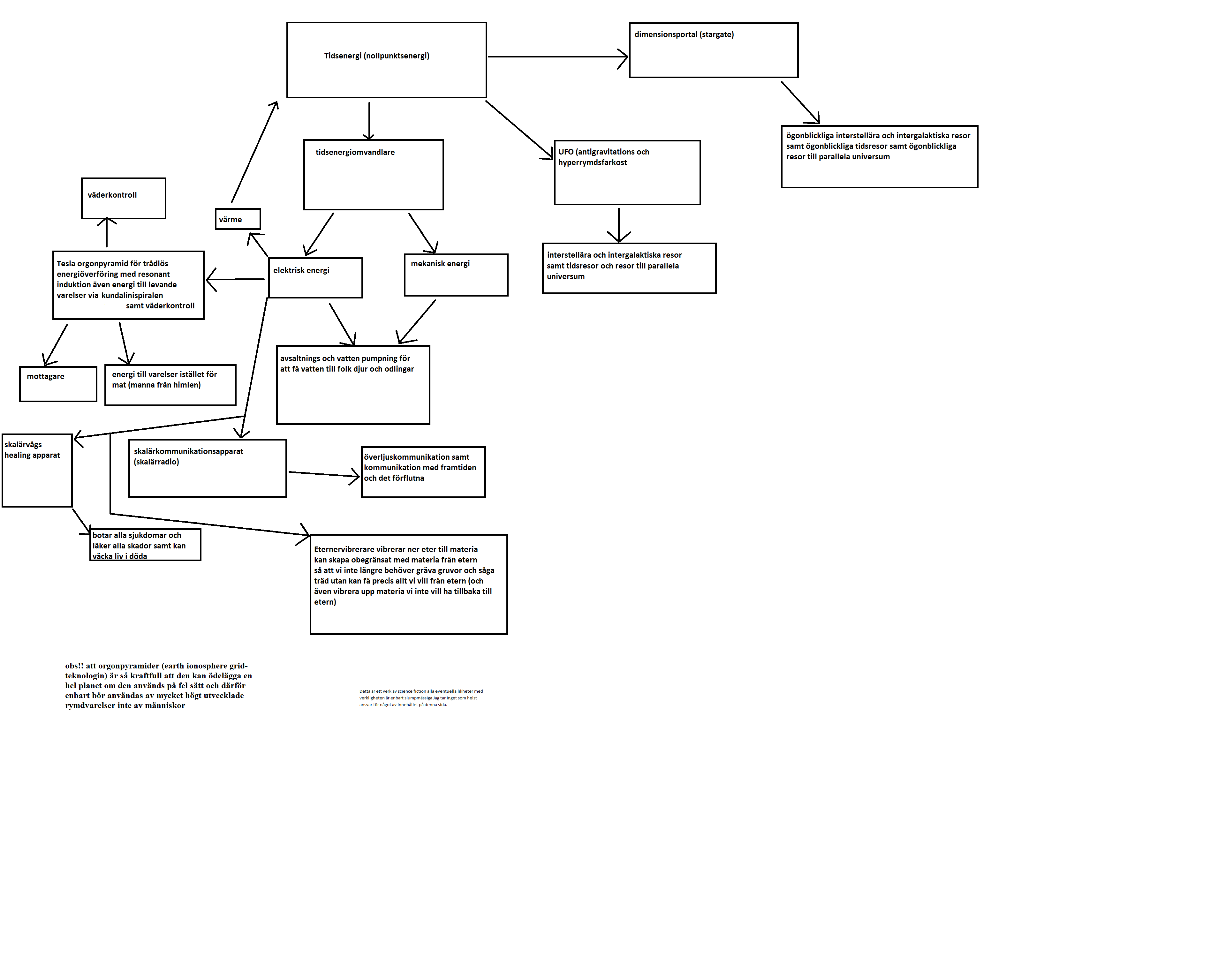<< < 13 | 14 | 15 | 16 | 17 > >>

Blogg

A Pure Java HPCC Grid Architecture

Current Research in Gravito-Electromagnetic Space Propulsion

Stationary Dissipative Solitons of Model G

Sök på hemsidan

Kontakt